21cmEMU v3: Full Emulator with 2D Power Spectrum
This tutorial demonstrates usage of 21cmEMUv3 emulator, including:
1D Summaries: 21-cm PS (\(\Delta^2_{21} (k)\) [mK\(^2\)]), global brightness temperature (\(\overline{T}_b\)), neutral fraction (\(\overline{x}_{\mathrm{HI}}\)), spin temperature (\(T_s\)), UV luminosity functions (UVLFs), and optical depth (\(\tau_e\))
2D Power Spectrum: The 21-cm power spectrum \(\Delta^2(k_\perp, k_\parallel)\) [mK\(^2\)] emulated by a diffusion model
Uncertainty Quantification: Variance estimation from multiple diffusion model samples
The v3 emulator uses:
An LSTM-based encoder-decoder architecture for 1D summaries
A score-based diffusion model architecture for the 2D power spectrum.
Requirements: This tutorial assumes a GPU is available for 2D PS emulation.
If you use this emulator in your work, please cite Breitman+26 (arXiv: 2606.00219).
[1]:
import numpy as np
import h5py
import matplotlib.pyplot as plt
from matplotlib import rcParams
import matplotlib.patches as mpatches
from matplotlib.lines import Line2D


rcParams.update({'font.size': 14})

from py21cmemu import Emulator
/home/dbreitman/.conda/envs/pytorch_env/lib/python3.10/site-packages/torch/utils/_pytree.py:185: FutureWarning: optree is installed but the version is too old to support PyTorch Dynamo in C++ pytree. C++ pytree support is disabled. Please consider upgrading optree using `python3 -m pip install --upgrade 'optree>=0.13.0'`.
  warnings.warn(
1. Load Test Databases
We load the test databases containing simulation outputs to compare against emulator predictions.
[2]:
# Load the 1D summaries test set
test_1d_path = 'test_database.h5'

with h5py.File(test_1d_path, 'r') as f:
    print("Test set keys:", list(f.keys()))

    # Input parameters (11 astrophysical params)
    test_params = np.array(f['input_params'])

    # 1D summaries
    test_xHI = np.array(f['xHI'])
    test_Tb = np.array(f['Tb'])
    test_Ts = np.array(f['Ts'])
    test_tau = np.array(f['tau'])
    test_PS_1D = np.array(f['PS_1D_seeds']) # shape is (Nparams, Nseeds, Nz, Nk)
    PS_redshifts = np.array(f['PS_redshifts'])
    k = np.array(f["k"])
    # UVLFs: (N, 7 z-bins, 60 magnitudes)
    test_LFs_raw = np.array(f['UVLFs'])

    # Axes
    redshifts = np.array(f['redshifts'])
    M_UV_all = np.array(f['M_UV'])
    LF_zs = np.array(f['UVLF_redshifts'])
    limits = np.array(f["limits"])
    ap = np.array(f["astro_param_keys"])

# Filter valid samples (no NaN inputs)
valid_mask = ~np.isnan(test_params.mean(axis=1))
print(f"Valid samples: {valid_mask.sum()} / {len(test_params)}")

test_params = test_params[valid_mask]
test_xHI = test_xHI[valid_mask]
test_Tb = test_Tb[valid_mask]
test_Ts = test_Ts[valid_mask]
test_tau = test_tau[valid_mask]
test_LFs_raw = test_LFs_raw[valid_mask]
test_PS_1D = test_PS_1D[valid_mask]
m = np.logical_and(M_UV_all < -10, M_UV_all > -20)
# Trim UVLFs to M_UV in [-20, -10]
M_UV = M_UV_all[m]  # Crop to 30 magnitudes
test_LFs = test_LFs_raw[:, :, m]  # (N, 7, 30)

print("\nData shapes:")
print(f"  Params: {test_params.shape}")
print(f"  xHI: {test_xHI.shape}")
print(f"  Tb: {test_Tb.shape}")
print(f"  Ts: {test_Ts.shape}")
print(f"  tau: {test_tau.shape}")
print(f"  UVLFs: {test_LFs.shape}")
print(f"  Redshifts: {redshifts.shape}")
Test set keys: ['M_UV', 'PS_1D_seeds', 'PS_redshifts', 'Tb', 'Ts', 'UVLF_redshifts', 'UVLFs', 'astro_param_keys', 'astro_param_labels', 'input_params', 'k', 'limits', 'redshifts', 'tau', 'xHI']
Valid samples: 80 / 80

Data shapes:
  Params: (80, 11)
  xHI: (80, 93)
  Tb: (80, 93)
  Ts: (80, 93)
  tau: (80,)
  UVLFs: (80, 7, 30)
  Redshifts: (93,)
[3]:
logged = [0,3,5,6,7,8]
for key, lim, idx in zip(ap, limits, range(len(ap))):
    print(key, lim, np.round(np.min(test_params[...,idx]),2), np.round(np.max(test_params[...,idx]),2))
b'F_STAR10' [-2.  -0.5] -1.81 -0.57
b'ALPHA_STAR' [0. 1.] 0.2 0.81
b't_STAR' [0.01 1.  ] 0.09 0.96
b'F_ESC10' [-3.  0.] -2.31 -0.05
b'ALPHA_ESC' [-1.  1.] -0.8 0.99
b'F_STAR7_MINI' [-4. -1.] -3.89 -1.1
b'F_ESC7_MINI' [-3. -1.] -2.89 -1.02
b'L_X' [38. 43.] 38.39 42.75
b'L_X_MINI' [39. 44.] 39.14 43.14
b'NU_X_THRESH' [ 100. 1500.] 118.92 1146.18
b'SIGMA_8' [0.75 0.85] 0.79 0.84
Load 2D Power Spectrum Test Database
The 2D PS test database contains power spectra computed at multiple redshifts.
Note: If the 2D PS test database is not available, the PS comparison sections will use emulator properties for k-grids and generate predictions without ground truth comparison.
[86]:
import os

# Try to load the 2D PS test database
test_ps2d_path = 'ps_2d_test_subsample.h5'
HAS_PS2D_DB = os.path.exists(test_ps2d_path)

if HAS_PS2D_DB:
    with h5py.File(test_ps2d_path, 'r') as f:
        print("2D PS test set keys:", list(f.keys()))

        ps_params = np.array(f['input_params'])
        ps_redshifts_all = np.array(f['redshifts'])
        kperp = np.array(f['kperp'])
        kpar = np.array(f['kpar_64'])  # 32 kpar bins

        # 2D PS: seeds (individual realisations) and means (averaged over seeds)
        ps_2d_seeds = np.array(f['PS_2D_64_seeds'])
        ps_2d_means = np.array(f['PS_2D_64_means'])

    # Select a subset of redshifts for 2D PS emulation (to save time)
    n_z_subset = 10
    z_indices = np.linspace(0, len(ps_redshifts_all) - 1, n_z_subset, dtype=int)
    ps_redshifts = ps_redshifts_all[z_indices]

    # Also subset the 2D PS data to match
    ps_2d_means = ps_2d_means[:, z_indices]
    ps_2d_seeds = ps_2d_seeds[:, z_indices]

    print("\n2D PS data shapes:")
    print(f"  Params: {ps_params.shape}")
    print(f"  All redshifts: {ps_redshifts_all.shape}")
    print(f"  Selected redshifts ({n_z_subset}): {ps_redshifts.shape}")
    print(f"  Selected z values: {ps_redshifts}")
    print(f"  kperp: {kperp.shape}")
    print(f"  kpar: {kpar.shape}")
    print(f"  PS seeds (subsetted): {ps_2d_seeds.shape}")
    print(f"  PS means (subsetted): {ps_2d_means.shape}")
else:
    print("2D PS test database not found.")
    print("PS sections will use emulator properties and test params from 1D database.")
    print("\nTo download the 2D PS test database, see the 21cmEMU documentation.")
    ps_params = test_params  # Use same params as 1D test
    ps_redshifts = None  # Will use emulator defaults
    ps_2d_means = None
    ps_2d_seeds = None
    kperp = None  # Will use emulator properties
    kpar = None   # Will use emulator properties
2D PS test set keys: ['N_modes', 'PS_2D_64_means', 'PS_2D_64_seeds', 'fnames', 'input_params', 'kpar_64', 'kperp', 'limits', 'param_keys', 'param_labels', 'redshifts']

2D PS data shapes:
  Params: (100, 11)
  All redshifts: (32,)
  Selected redshifts (10): (10,)
  Selected z values: [ 5.50105421  6.46050805  7.59002262  9.40138137 11.04865309 13.6898716
 16.07786482 19.92643643 23.39700184 28.98670671]
  kperp: (32,)
  kpar: (64,)
  PS seeds (subsetted): (100, 10, 32, 64)
  PS means (subsetted): (100, 10, 32, 64)
2. Initialize the v3 Emulator
We load the MH emulator without 2D PS emulation enabled for now, so set emulate_2d_ps=False:
[4]:
emu = Emulator(emulator='mh', emulate_2d_ps=False)

print(f"Emulator initialized: {emu.which_emulator}")
print(f"PS emulation: {emu.emulate_2d_ps}")
print("\nAvailable properties:")
print(f"  Redshifts: {emu.properties.zs.shape}")
print(f"  PS redshifts: {emu.properties.PS_zs.shape}")
print(f"  kperp: {emu.properties.kperp.shape}")
print(f"  kpar: {emu.properties.kpar.shape}")
Emulator initialized: mcg
PS emulation: False

Available properties:
  Redshifts: (93,)
  PS redshifts: (32,)
  kperp: (32,)
  kpar: (64,)
3. Run Emulator Predictions
We run the emulator on a subset of test parameters.
[5]:
# Select a subset for demonstration (to save time)
n_samples = min(10, len(test_params))
idx = np.random.choice(len(test_params), n_samples, replace=False)
idx = np.sort(idx)

params_subset = test_params[idx]

print(f"Running emulator on {n_samples} samples...")

# Run prediction with EM sampling for 2D PS
normed_params, output, errors = emu.predict(
    params_subset,
    verbose=True,
    ps_sampling_method='ode',  # probability flow ODE or Euler-Maruyama 'em' sampling supported
    n_realisations=10,  # Number of diffusion realisations

)

print(f"\nOutput keys: {list(output.keys())}")
Running emulator on 10 samples...

Output keys: ['Tb', 'xHI', 'Ts', 'tau', 'UVLFs', 'PS', 'PS_2D', 'PS_2D_samples', 'PS_2D_std', 'PS_2D_redshifts']
[6]:
# Extract emulated outputs
emu_xHI = output['xHI'].value
emu_Tb = output['Tb'].value
emu_Ts = output['Ts'].value
emu_tau = output['tau'].value
emu_UVLFs = output['UVLFs'].value
emu_PS = output["PS"].value

# Extract true outputs for comparison
true_xHI = test_xHI[idx]
true_Tb = test_Tb[idx]
true_Ts = test_Ts[idx]
true_tau = test_tau[idx]
true_UVLFs = test_LFs[idx]
true_PS = test_PS_1D[idx]

print(f"Emulated xHI shape: {emu_xHI.shape}")
print(f"Emulated Tb shape: {emu_Tb.shape}")
print(f"Emulated Ts shape: {emu_Ts.shape}")
print(f"Emulated tau shape: {emu_tau.shape}")
print(f"Emulated UVLFs shape: {emu_UVLFs.shape}")
Emulated xHI shape: (10, 93)
Emulated Tb shape: (10, 93)
Emulated Ts shape: (10, 93)
Emulated tau shape: (10,)
Emulated UVLFs shape: (10, 7, 30)
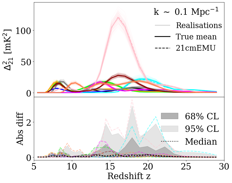
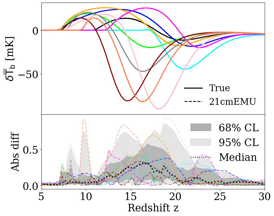
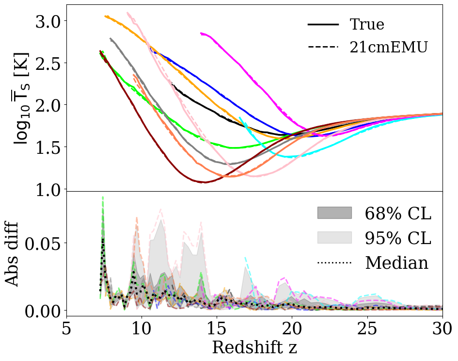
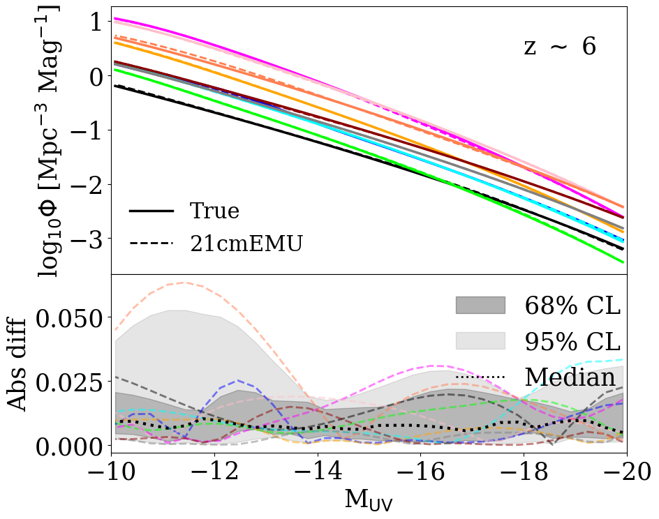
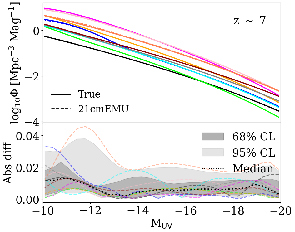
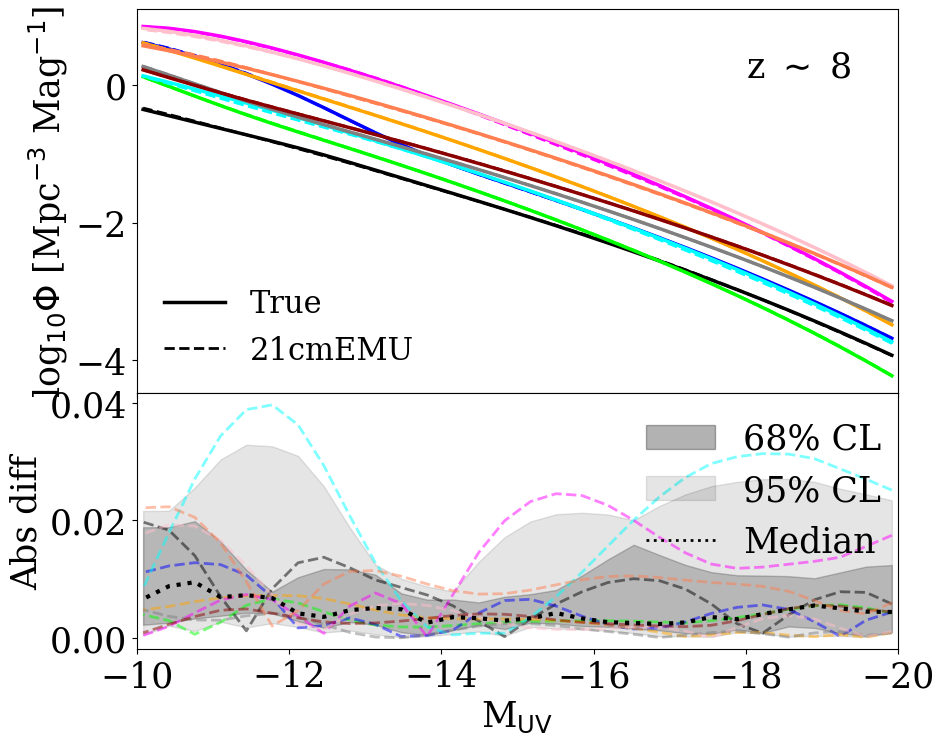
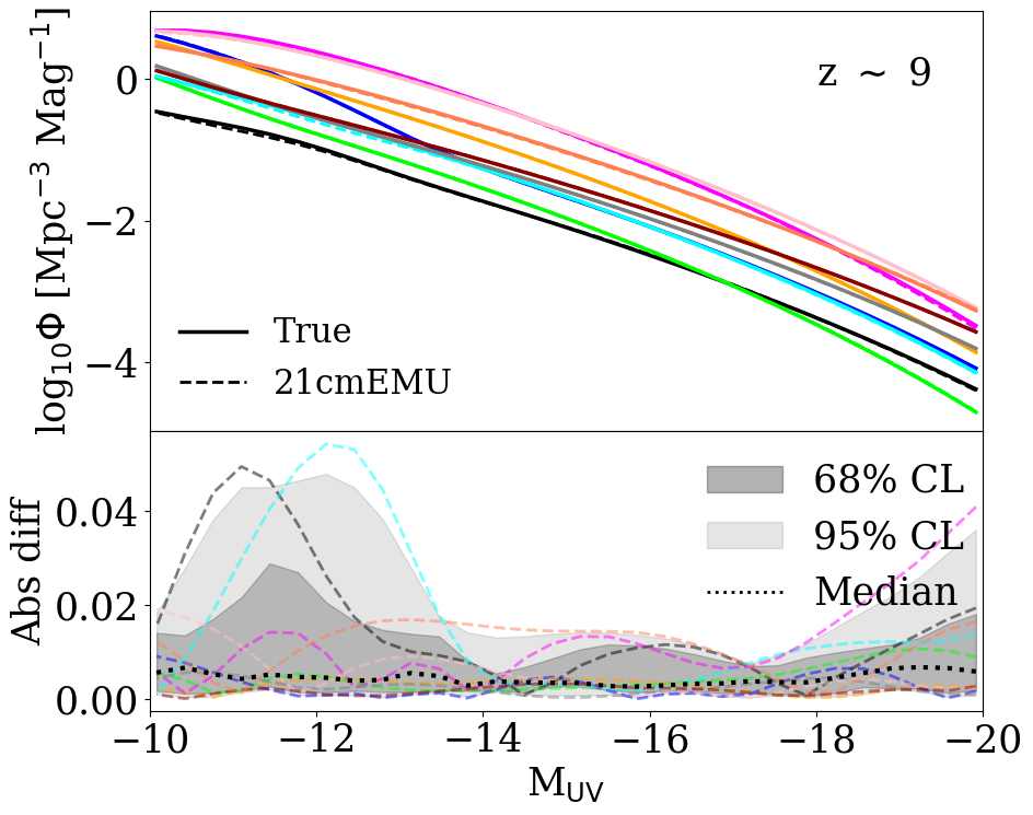
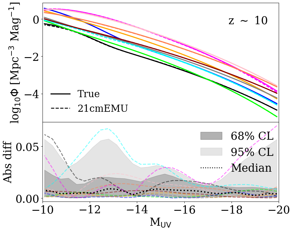
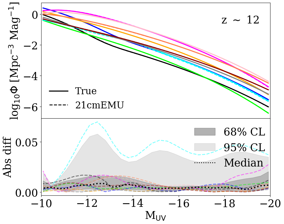
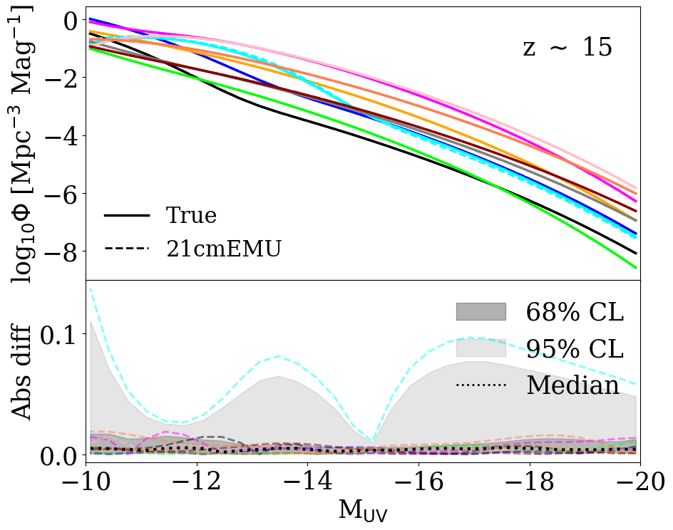
4. Compare 1D Summaries: True vs Emulated
We plot several test samples comparing the true (simulation) values with emulated predictions.
[7]:
def plot_true_vs_emu(x, y_true, y_emu, x_label,
                     y_label, y_diff = None,
                     xlims = None, ylims = None,
                     N = 10, offset = 0,
                     plot_realisations=False, FE=False,
                     logFE=False, floor = 1e-2,
                     cs = None, leg_loc = (0.5,0.5), cl_leg_loc = (0.6,0.5)):
    if cs is None:
        cs = ['k','lime','b', 'orange', 'cyan', 'magenta', 'grey', 'pink', 'darkred', 'coral']
    if plot_realisations:
        y_mean = np.nanmean(y_true, axis=1)          # (N_param, len(x)) — true mean
    else:
        y_mean = y_true
    if y_diff is None:
        if not FE:
            y_diff = np.abs(y_mean - y_emu)               # (N_param, len(x)) — mean vs emu residual
        else:
            if logFE:
                y_diff = log10_fractional_error(y_mean, y_emu, floor_log=floor)
            else:
                y_diff = fractional_error(y_mean, y_emu, floor=floor)

    fig, axs = plt.subplots(nrows=2, ncols=1, sharex=True, figsize=(10, 8),
                            gridspec_kw=dict(height_ratios=[3, 2], hspace=0))
    axs = axs.flatten()

    diff_err_z = np.nanpercentile(y_diff, [2.5, 16, 50, 84, 97.5], axis=0)
    for i, c in zip(range(N), cs):
        idx = i + offset
        last = (i == N - 1)
        if plot_realisations:
            # Individual realisations — thin, semi-transparent
            for j in range(y_true.shape[1]):
                axs[0].plot(x, y_true[idx, j], lw=0.7, color=c, alpha=0.15)

        # True mean — thick solid
        axs[0].plot(x, y_mean[idx], lw=2.5, color=c)

        # Emulator prediction — dashed
        axs[0].plot(x, y_emu[idx], lw=2, ls='--', color=c)

        # Per-parameter residual (true mean vs emu) in lower panel
        if not FE:
            axs[1].plot(x, np.abs(y_mean[idx] - y_emu[idx]), ls='--', alpha=0.5, lw=2, color=c)
        else:
            if logFE:
                axs[1].plot(x, log10_fractional_error(y_mean[idx], y_emu[idx], floor_log=floor), ls='--', alpha=0.5, lw=2, color=c)
            else:
                axs[1].plot(x, fractional_error(y_mean[idx], y_emu[idx], floor=floor), ls='--', alpha=0.5, lw=2, color=c)

    if plot_realisations:
        legend_handles = [
            Line2D([0], [0], color='k', lw=0.7, alpha=0.6, label='Realisations'),
            Line2D([0], [0], color='k', lw=2.5, label='True mean'),
            Line2D([0], [0], color='k', lw=2, ls='--', label='21cmEMU'),
        ]
    else:
        legend_handles = [
            Line2D([0], [0], color='k', lw=2.5, label='True mean' if plot_realisations else 'True'),
            Line2D([0], [0], color='k', lw=2, ls='--', label='21cmEMU'),
        ]
    axs[0].legend(handles=legend_handles, loc=leg_loc, frameon=False, fontsize = 22)
    axs[1].plot(x, diff_err_z[2], ls=':', lw=3, color='k', label='Median')
    axs[1].fill_between(x, diff_err_z[1], diff_err_z[3], color='k', alpha=0.2, label='68% CI')
    axs[1].fill_between(x, diff_err_z[0], diff_err_z[4], color='k', alpha=0.1, label='95% CI')

    handles = [mpatches.Patch(color='k', label='68% CL', alpha=0.3),
               mpatches.Patch(color='k', label='95% CL', alpha=0.1),
#                mpatches.Patch(color='r', label='Mean PS', alpha=0.1),
               Line2D([0], [0], color='k', lw=2, ls=':', label='Median'),]
    if cl_leg_loc is not None:
        axs[1].legend(handles=handles, loc=cl_leg_loc, frameon=False)

    axs[0].set_ylabel(y_label)
    axs[1].set_ylabel(r'Abs diff' if not FE else 'FE (%)')
    axs[1].set_xlabel(x_label)
    if xlims is not None:
        plt.xlim(xlims[0], xlims[1])
    else:
        plt.xlim(min(x), max(x))
    if ylims is not None:
        axs[0].set_ylim(ylims[0], ylims[1])
#         axs[1].set_ylim(-0.1,0.1)
        axs[0].set_yscale('log')
    return fig
[8]:
def fractional_error(true, pred, floor=1e-2):
    """Compute fractional error in percent
    with floor to avoid division by small numbers.


    FE = |true - pred| / max(true, floor) * 100
    """
    denom = true.copy()
    denom[np.abs(denom) < floor] = floor
    return np.abs((true - pred) / denom) * 100.0


def log10_fractional_error(true, pred, floor_log=1e-2):
    """FE on log10 PS: |log10(true) - log10(pred)| / max(|log10(true)|, floor_log) * 100.

    Uses |log10(true)| as denominator with a floor to handle PS ~ 1 (log10 ~ 0).
    Default floor_log=1e-2: pixels where |log10(PS)| < 1e-2 use 1e-2 as denominator.
    """
    log_true = np.log10(true)
    log_pred = np.log10(pred)
    denom = np.abs(log_true)
    denom[denom < floor_log] = floor_log
    return np.abs((log_true - log_pred) / denom) * 100.0
[9]:
from matplotlib import rcParams
rcParams.update({"font.size":25, "font.family": 'serif'})
k_idx = 11
fig = plot_true_vs_emu(PS_redshifts, true_PS[...,k_idx], emu_PS[...,k_idx], r'Redshift z', r'$\Delta^2_{21}$ [mK$^2$]',
                 xlims = [5., 30],
#                        y_diff = diff_random[...,k_idx],
                       plot_realisations=True,
                leg_loc = (0.62,0.44),
                      cl_leg_loc = (0.65, 0.17))
axs = fig.get_axes()
axs[0].text(0.8, 0.9,
            "k $\sim$ " + str(np.round(k[k_idx],1)) +" Mpc$^{-1}$",
            horizontalalignment='center',
            verticalalignment='center',
            transform=axs[0].transAxes)

# diff_err_z = np.nanpercentile(diff_mean[...,k_idx], [2.5, 16, 50, 84, 97.5], axis=0)
# axs[1].fill_between(PS_redshifts, diff_err_z[1], diff_err_z[3], color='r', alpha=0.2, label='Mean')
# axs[1].fill_between(PS_redshifts, diff_err_z[0], diff_err_z[4], color='r', alpha=0.1,)
# axs[1].plot(PS_redshifts, diff_err_z[2], ls=':', lw=3, color='r')
plt.tight_layout()
# plt.savefig("PS_true_vs_emu.pdf")
plt.show()
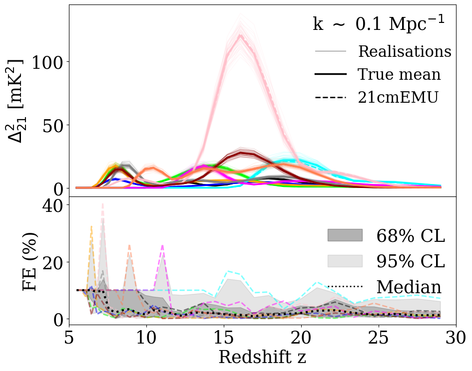
[10]:
from matplotlib import rcParams
rcParams.update({"font.size":25, "font.family": 'serif'})
k_idx = 11
fig = plot_true_vs_emu(PS_redshifts, true_PS[...,k_idx], emu_PS[...,k_idx], r'Redshift z', r'$\Delta^2_{21}$ [mK$^2$]',
                 xlims = [5., 30],
#                        y_diff = fe_random[...,k_idx],
                       FE=True, floor = 0.1, logFE=False,
                       plot_realisations=True,
                leg_loc = (0.62,0.44),
                      cl_leg_loc = (0.65, 0.17))
axs = fig.get_axes()
axs[0].text(0.8, 0.9,
            "k $\sim$ " + str(np.round(k[k_idx],1)) +" Mpc$^{-1}$",
            horizontalalignment='center',
            verticalalignment='center',
            transform=axs[0].transAxes)
# diff_err_z = np.nanpercentile(PS_mean_fe[...,k_idx], [2.5, 16, 50, 84, 97.5], axis=0)
# axs[1].fill_between(PS_redshifts, diff_err_z[1], diff_err_z[3], color='r', alpha=0.2, label='Mean')
# axs[1].fill_between(PS_redshifts, diff_err_z[0], diff_err_z[4], color='r', alpha=0.1,)
# axs[1].plot(PS_redshifts, diff_err_z[2], ls=':', lw=3, color='r')
# axs[1].set_ylim(0,50)
plt.tight_layout()
# plt.savefig("PS_true_vs_emu_FE.png")
plt.show()
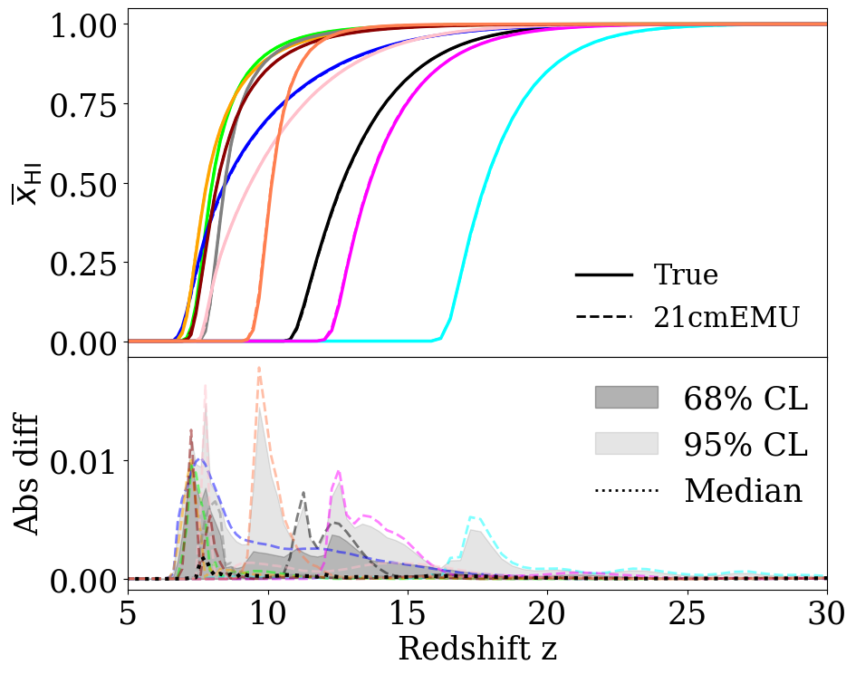
[11]:
from matplotlib import rcParams
rcParams.update({"font.size":25, "font.family": 'serif'})
fig = plot_true_vs_emu(redshifts, true_xHI, emu_xHI, r'Redshift z', r'$\overline{x}_{\rm HI}$',
                       plot_realisations = False,
                 xlims = [5., 30],
                leg_loc = None,
                cl_leg_loc = (0.65, 0.3))

plt.tight_layout()
# plt.savefig("xHI_true_vs_emu.pdf", format = "pdf")
plt.show()
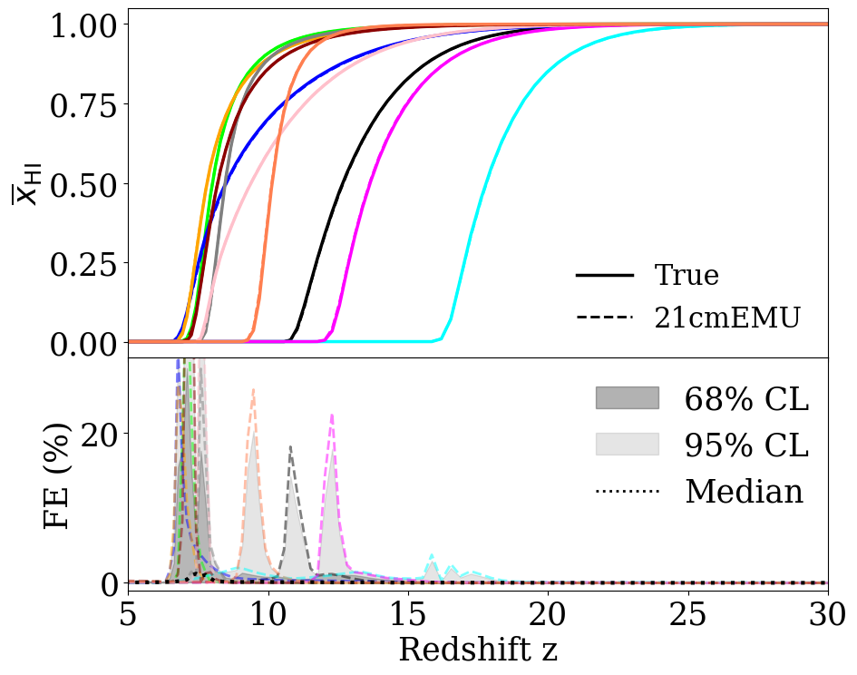
[12]:
from matplotlib import rcParams
rcParams.update({"font.size":25, "font.family": 'serif'})
fig = plot_true_vs_emu(redshifts, true_xHI, emu_xHI, r'Redshift z', r'$\overline{x}_{\rm HI}$',
                       plot_realisations = False, FE=True,
                 xlims = [5., 30],
                leg_loc = None,
                cl_leg_loc = (0.65, 0.3))
axs = fig.get_axes()
axs[1].set_ylim(-1,30)
plt.tight_layout()
# plt.savefig("xHI_true_vs_emu_FE.pdf")
plt.show()
[13]:
from matplotlib import rcParams
rcParams.update({"font.size":25, "font.family": 'serif'})
fig = plot_true_vs_emu(redshifts, true_Tb, emu_Tb,
                       r'Redshift z', r'$ \delta\overline{\rm{T}}_{\rm b}$ [mK]',
                       plot_realisations = False,
                 xlims = [5., 30],
                leg_loc = None,
                cl_leg_loc = (0.65, 0.3))

plt.tight_layout()
# plt.savefig("Tb_true_vs_emu.pdf", format = "pdf")
plt.show()
[14]:
from matplotlib import rcParams
rcParams.update({"font.size":25, "font.family": 'serif'})
fig = plot_true_vs_emu(redshifts, np.log10(true_Ts), np.log10(emu_Ts), r'Redshift z', r'$\log_{10}\overline{\rm{T}}_{\rm S}$ [K]',
                       plot_realisations = False,
                 xlims = [5., 30],
                leg_loc = None,
                cl_leg_loc = (0.65, 0.3))

plt.tight_layout()
# plt.savefig("Ts_true_vs_emu.pdf", format = "pdf")
plt.show()
/home/dbreitman/.conda/envs/pytorch_env/lib/python3.10/site-packages/numpy/lib/nanfunctions.py:1563: RuntimeWarning: All-NaN slice encountered
  return function_base._ureduce(a,
[15]:
true_UVLFs.shape, emu_UVLFs.shape, M_UV.shape
[15]:
((10, 7, 30), (10, 7, 30), (30,))
[16]:
for i in range(len(LF_zs)):
    fig = plot_true_vs_emu(M_UV, true_UVLFs[:,i,:], emu_UVLFs[:,i,:],
                     r'M$_{\rm UV}$', r'log$_{10}\Phi$ [Mpc$^{-3}$ Mag$^{-1}$]',
                     xlims = [-10, -20],
                           plot_realisations=False,
                      leg_loc = "lower left", cl_leg_loc = (0.65, 0.3))
    axs = fig.get_axes()
    axs[0].text(0.87, 0.85,
                r"z $\sim$"+f" {LF_zs[i]:n} ",
                horizontalalignment='center',
                verticalalignment='center',
                transform=axs[0].transAxes)
    plt.tight_layout()
#     plt.savefig(f"UVLFs_true_vs_emu{LF_zs[i]:n}.pdf", format = "pdf")
    plt.show()
[17]:
cs = ['k','lime','b', 'orange', 'cyan', 'magenta', 'grey', 'pink', 'darkred', 'coral']
[18]:
tau_bins = np.linspace(min(true_tau), np.nanpercentile(true_tau,95), 3)
tau_binned_fe = np.zeros(len(tau_bins))
tau_binned_fe_68 = np.zeros((len(tau_bins),2))
tau_binned_fe_95 = np.zeros((len(tau_bins),2))

tau_binned = np.zeros(len(tau_bins))
tau_binned_68 = np.zeros((len(tau_bins),2))
tau_binned_95 = np.zeros((len(tau_bins),2))
[19]:
tau_diff = abs((emu_tau - true_tau))
tau_frac_err = abs((emu_tau - true_tau) / true_tau) * 100.
[20]:
for i in range(len(tau_bins)-1):
    mask = np.logical_and(true_tau >= tau_bins[i], true_tau < tau_bins[i+1])
    low1, low, med, high, high1 = np.nanpercentile(tau_frac_err[mask], [2.5, 16,50,84, 97.5])
    tau_binned_fe[i] = med
    tau_binned_fe_68[i,:] = [low, high]
    tau_binned_fe_95[i,:] = [low1, high1]

    low1, low, med, high, high1 = np.nanpercentile(tau_diff[mask], [2.5, 16,50,84, 97.5])
    tau_binned[i] = med
    tau_binned_68[i,:] = [low, high]
    tau_binned_95[i,:] = [low1, high1]
[21]:
tau_frac_err2 = abs((emu_tau - true_tau) / true_tau) * 100.
tau_diff2 = abs(emu_tau - true_tau)
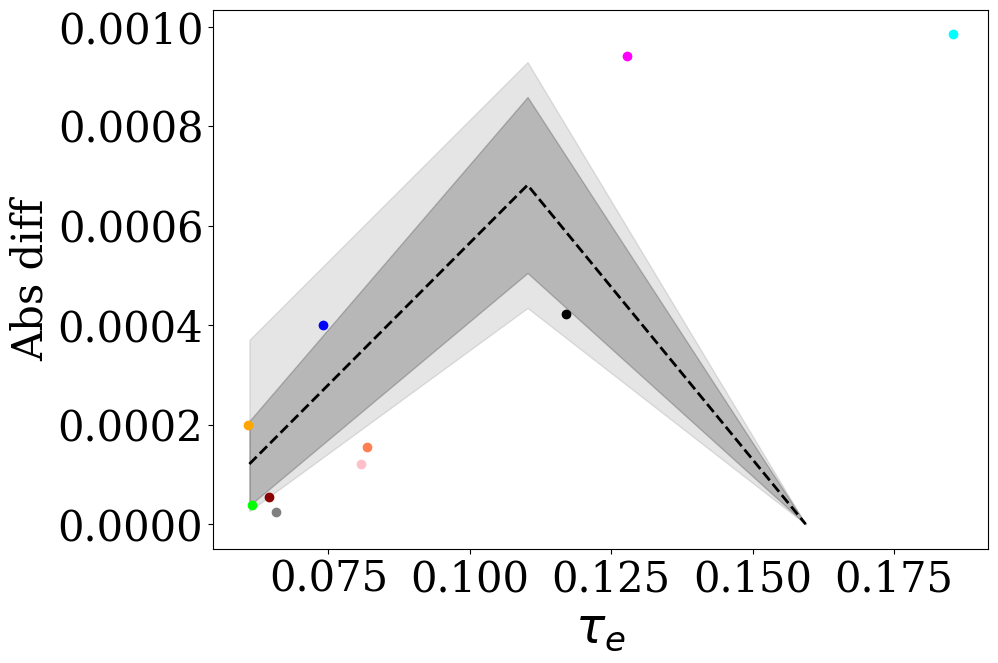
[22]:
plt.figure(figsize=(10,7))
rcParams.update({'font.size': 30})
plt.plot(tau_bins, tau_binned, color = 'k', lw = 2, ls = '--')
plt.fill_between(tau_bins, tau_binned_68[:,0], tau_binned_68[:,1], color = 'k', alpha = 0.2)
plt.fill_between(tau_bins, tau_binned_95[:,0], tau_binned_95[:,1], color = 'k', alpha = 0.1)
for i in range(10):
    plt.scatter(emu_tau[i], tau_diff2[i], color = cs[i], marker = 'o', zorder = 2)
#plt.scatter(10**tau_true, tau_frac_err, alpha = 0.1)
plt.xlabel(r'$\tau_e$', fontsize=35)
handles = [mpatches.Patch(color='k', label='68% CI', alpha = 0.1),
          mpatches.Patch(color='k', label='95% CI', alpha = 0.3),
          ]
#plt.legend(handles=handles, loc = (0.05,0.7), frameon = False, fontsize = 20)
plt.ylabel('Abs diff')
# plt.savefig('tau_binned.png', dpi = 300, bbox_inches = "tight")
plt.show()
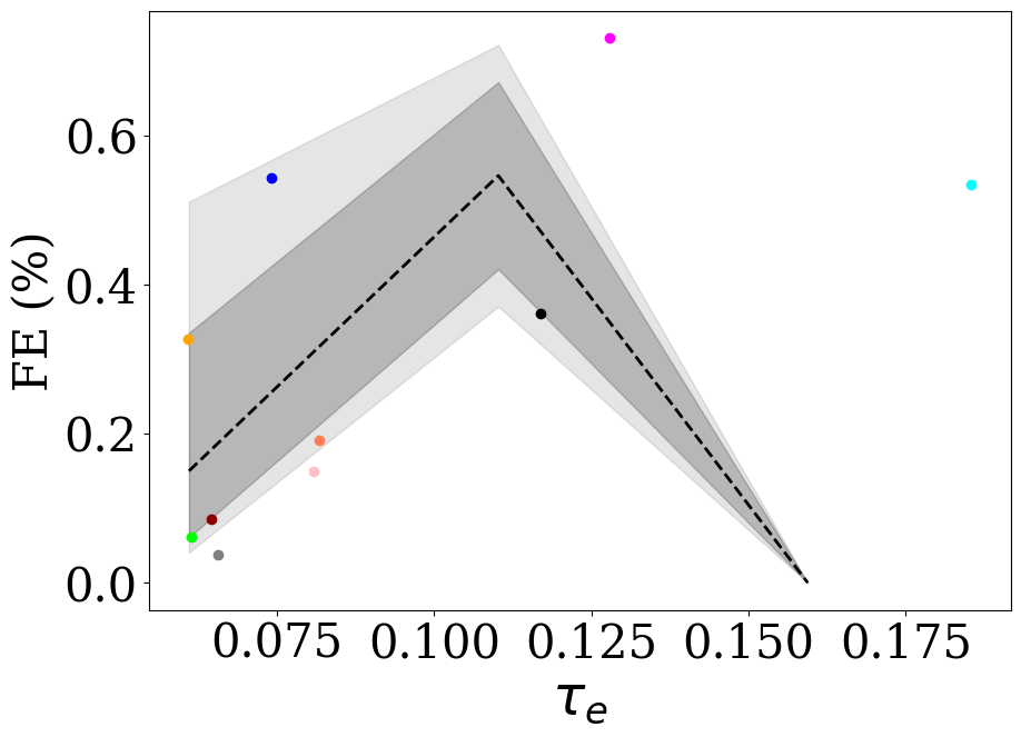
[23]:
plt.figure(figsize=(10,7))
rcParams.update({'font.size': 30})
plt.plot(tau_bins, tau_binned_fe, color = 'k', lw = 2, ls = '--')
plt.fill_between(tau_bins, tau_binned_fe_68[:,0], tau_binned_fe_68[:,1], color = 'k', alpha = 0.2)
plt.fill_between(tau_bins, tau_binned_fe_95[:,0], tau_binned_fe_95[:,1], color = 'k', alpha = 0.1)
for i in range(10):
    plt.scatter(emu_tau[i], tau_frac_err2[i], color = cs[i], marker = 'o', zorder = 2)
#plt.scatter(10**tau_true, tau_frac_err, alpha = 0.1)
plt.xlabel(r'$\tau_e$', fontsize=35)
handles = [mpatches.Patch(color='k', label='68% CI', alpha = 0.1),
          mpatches.Patch(color='k', label='95% CI', alpha = 0.3),
          ]
#plt.legend(handles=handles, loc = (0.05,0.7), frameon = False, fontsize = 20)
plt.ylabel('FE (%)')
# plt.savefig('tau_binned_FE.pdf', dpi = 300, bbox_inches = "tight")
plt.show()
Compute Fractional Errors
[24]:
# Compute FEs
fe_xHI = fractional_error(true_xHI, emu_xHI, floor=0.01)
fe_Tb = fractional_error(true_Tb, emu_Tb, floor=5.0)  # 5 mK floor for Tb
fe_Ts = fractional_error(np.log10(true_Ts + 1e-3), np.log10(emu_Ts + 1e-3), floor=0.01)
fe_tau = fractional_error(true_tau, emu_tau, floor=0.01)

print("Fractional Error Statistics (%)")
print("=" * 50)
for name, fe in [('xHI', fe_xHI), ('Tb', fe_Tb), ('Ts', fe_Ts), ('tau', fe_tau)]:
    finite = fe[np.isfinite(fe)]
    print(f"{name:8s}: median={np.median(finite):6.2f}%  "
          f"68th={np.percentile(finite, 68):6.2f}%  "
          f"95th={np.percentile(finite, 95):6.2f}%")
Fractional Error Statistics (%)
==================================================
xHI     : median=  0.03%  68th=  0.09%  95th=  2.08%
Tb      : median=  0.60%  68th=  0.91%  95th=  4.53%
Ts      : median=  0.18%  68th=  0.37%  95th=  1.22%
tau     : median=  0.26%  68th=  0.38%  95th=  0.65%
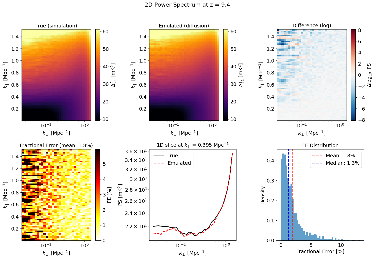
5. 2D Power Spectrum Emulation
The v3 emulator uses a score-based diffusion model to emulate the 2D power spectrum. This allows:
Probabilistic predictions with multiple samples
Variance and covariance estimation from the sample distribution
Two sampling methods: Euler-Maruyama (EM) and Probability-flow ODE
[26]:
# Select a few parameters for 2D PS demonstration
n_ps_samples = 2
ps_test_idx = np.random.choice(len(ps_params), n_ps_samples, replace=False)

# Prepare parameters - we need to combine astro params with redshift
# The emulator expects 11 astro params; redshift is added internally
ps_test_params = ps_params[ps_test_idx]

print(f"Testing 2D PS on {n_ps_samples} parameter sets")
print(f"Parameter shape: {ps_test_params.shape}")
if ps_redshifts is not None:
    print(f"Using {len(ps_redshifts)} test set redshifts: {ps_redshifts}")

# Run with more samples for variance estimation
# Pass ps_redshifts to match the test set redshifts
_, ps_output, ps_errors = emu.predict(
    ps_test_params,
    verbose=True,
    ps_2d_redshifts=ps_redshifts,  # Use test set redshifts for comparison
    ps_sampling_method='ode',
    n_ps_batch=5,
    n_realisations=100  # More samples for better variance estimate
)
Testing 2D PS on 2 parameter sets
Parameter shape: (2, 11)
Using 10 test set redshifts: [ 5.50105421  6.46050805  7.59002262  9.40138137 11.04865309 13.6898716
 16.07786482 19.92643643 23.39700184 28.98670671]
Computing 2D PS: 100%|██████████| 4/4 [01:55<00:00, 28.93s/batch]
[35]:
# Access PS outputs
# PS_2D shape: (n_params, n_redshifts, 32, 64) - median of diffusion samples
ps_emu = 10**ps_output['PS_2D'].value  # Delat_{21}^2 [mK^2] 2D PS median
print(f"Emulated 2D PS shape (median): {ps_emu.shape}")

# Get the actual redshifts used for 2D PS emulation
ps_emu_zs = output.PS_2D_redshifts if hasattr(output, 'PS_2D_redshifts') else ps_redshifts
print(f"2D PS redshifts: {ps_emu_zs}")

# Also access 1D PS from LSTM
ps_1d = ps_output['PS'].value
print(f"1D PS shape: {ps_1d.shape}")
Emulated 2D PS shape (median): (2, 10, 32, 64)
2D PS redshifts: [ 5.5         6.97446005  7.54906604  7.9582024   9.82883407 10.36152691
 10.63860385 16.66170964 19.52022545 24.10859229]
1D PS shape: (2, 32, 32)
[47]:
# Plot 2D PS comparison for one parameter set at one redshift
param_idx = 0
z_idx = 3  # Middle redshift in our subset (0 to n_z_subset-1)

# Get k-grids from emulator properties
kperp_emu = emu.properties.kperp
kpar_emu = emu.properties.kpar

if HAS_PS2D_DB and ps_2d_means is not None:
    # Get true PS from database (already subsetted to match ps_redshifts)
    true_ps_2d_sel = ps_2d_means[ps_test_idx]  # Shape: (n_ps_samples, n_z_subset, 32, 64)
    emu_ps_2d_sel = ps_emu  # Shape: (n_ps_samples, n_z_subset, 32, 64)

    print(f"True PS shape: {true_ps_2d_sel.shape}")
    print(f"Emulated PS shape: {emu_ps_2d_sel.shape}")
    print(f"Comparing at z = {ps_redshifts[z_idx]:.2f}")

    fig, axes = plt.subplots(2, 3, figsize=(15, 10))

    # True PS at selected redshift
    true_ps = true_ps_2d_sel[param_idx, z_idx]
    emu_ps = emu_ps_2d_sel[param_idx, z_idx]

    vmin = np.percentile(true_ps, 5)
    vmax = np.percentile(true_ps, 95)

    # Row 1: PS values
    im0 = axes[0, 0].pcolormesh(kperp_emu, kpar_emu, true_ps.T,
                                 vmin=vmin, vmax=vmax, cmap='inferno')
    axes[0, 0].set_title('True (simulation)', fontsize=14)
    axes[0, 0].set_xlabel(r'$k_\perp$ [Mpc$^{-1}$]')
    axes[0, 0].set_ylabel(r'$k_\parallel$ [Mpc$^{-1}$]')
    axes[0, 0].set_xscale('log')
    plt.colorbar(im0, ax=axes[0, 0], label=r'$\Delta^2_{21}$ [mK$^2$]')

    im1 = axes[0, 1].pcolormesh(kperp_emu, kpar_emu, emu_ps.T,
                                 vmin=vmin, vmax=vmax, cmap='inferno')
    axes[0, 1].set_title('Emulated (diffusion)', fontsize=14)
    axes[0, 1].set_xlabel(r'$k_\perp$ [Mpc$^{-1}$]')
    axes[0, 1].set_ylabel(r'$k_\parallel$ [Mpc$^{-1}$]')
    axes[0, 1].set_xscale('log')
    plt.colorbar(im1, ax=axes[0, 1], label=r'$\Delta^2_{21}$ [mK$^2$]')

    # Difference
    diff = emu_ps - true_ps
    vlim = np.max(np.abs(diff))
    im2 = axes[0, 2].pcolormesh(kperp_emu, kpar_emu, diff.T,
                                 vmin=-vlim, vmax=vlim, cmap='RdBu_r')
    axes[0, 2].set_title('Difference (log)', fontsize=14)
    axes[0, 2].set_xlabel(r'$k_\perp$ [Mpc$^{-1}$]')
    axes[0, 2].set_ylabel(r'$k_\parallel$ [Mpc$^{-1}$]')
    axes[0, 2].set_xscale('log')
    plt.colorbar(im2, ax=axes[0, 2], label=r'$\Delta \log_{10}$ PS')

    # Row 2: FE and 1D slices
    fe_ps = fractional_error(true_ps, emu_ps, floor=0.01)

    im3 = axes[1, 0].pcolormesh(kperp_emu, kpar_emu, fe_ps.T,
                                 vmin=0, vmax=min(100, np.percentile(fe_ps, 95)),
                                 cmap='hot_r')
    axes[1, 0].set_title(f'Fractional Error (mean: {np.mean(fe_ps):.1f}%)', fontsize=14)
    axes[1, 0].set_xlabel(r'$k_\perp$ [Mpc$^{-1}$]')
    axes[1, 0].set_ylabel(r'$k_\parallel$ [Mpc$^{-1}$]')
    axes[1, 0].set_xscale('log')
    plt.colorbar(im3, ax=axes[1, 0], label='FE [%]')

    # 1D slice along kperp (fixed kpar)
    kpar_slice_idx = 16  # Middle kpar
    axes[1, 1].plot(kperp_emu, true_ps[:, kpar_slice_idx], 'k-', lw=2, label='True')
    axes[1, 1].plot(kperp_emu, emu_ps[:, kpar_slice_idx], 'r--', lw=2, label='Emulated')
    axes[1, 1].set_xscale('log')
    axes[1, 1].set_yscale('log')
    axes[1, 1].set_xlabel(r'$k_\perp$ [Mpc$^{-1}$]')
    axes[1, 1].set_ylabel(r'PS [mK$^2$]')
    axes[1, 1].set_title(f'1D slice at $k_\\parallel$ = {kpar_emu[kpar_slice_idx]:.3f} Mpc$^{{-1}}$', fontsize=14)
    axes[1, 1].legend()

    # FE histogram
    axes[1, 2].hist(fe_ps.ravel(), bins=50, alpha=0.7, density=True)
    axes[1, 2].axvline(np.mean(fe_ps), color='r', ls='--', lw=2,
                       label=f'Mean: {np.mean(fe_ps):.1f}%')
    axes[1, 2].axvline(np.median(fe_ps), color='b', ls='--', lw=2,
                       label=f'Median: {np.median(fe_ps):.1f}%')
    axes[1, 2].set_xlabel('Fractional Error [%]')
    axes[1, 2].set_ylabel('Density')
    axes[1, 2].set_title('FE Distribution', fontsize=14)
    axes[1, 2].legend()

    plt.suptitle(f'2D Power Spectrum at z = {ps_redshifts[z_idx]:.1f}', fontsize=16, y=1.02)
    plt.tight_layout()
    plt.show()

else:
    # Without database, just show the emulated PS
    kperp_emu = emu.properties.kperp
    kpar_emu = emu.properties.kpar
    emu_ps = ps_emu[param_idx, z_idx]

    fig, axes = plt.subplots(1, 3, figsize=(15, 5))

    vmin = np.percentile(np.log10(emu_ps + 1e-10), 5)
    vmax = np.percentile(np.log10(emu_ps + 1e-10), 95)

    im0 = axes[0].pcolormesh(kperp_emu, kpar_emu, np.log10(emu_ps).T,
                              vmin=vmin, vmax=vmax, cmap='inferno')
    axes[0].set_title('Emulated 2D PS', fontsize=14)
    axes[0].set_xlabel(r'$k_\perp$ [Mpc$^{-1}$]')
    axes[0].set_ylabel(r'$k_\parallel$ [Mpc$^{-1}$]')
    axes[0].set_xscale('log')
    plt.colorbar(im0, ax=axes[0], label=r'$\Delta^2_{21}$ [mK$^2$]')

    # 1D slice along kperp (fixed kpar)
    kpar_slice_idx = 16  # Middle kpar
    axes[1].plot(kperp_emu, emu_ps[:, kpar_slice_idx], 'r-', lw=2, label='Emulated')
    axes[1].set_xscale('log')
    axes[1].set_yscale('log')
    axes[1].set_xlabel(r'$k_\perp$ [Mpc$^{-1}$]')
    axes[1].set_ylabel(r'PS [mK$^2$]')
    axes[1].set_title(f'1D slice at $k_\\parallel$ = {kpar_emu[kpar_slice_idx]:.3f} Mpc$^{{-1}}$', fontsize=14)
    axes[1].legend()

    # 1D slice along kpar (fixed kperp)
    kperp_slice_idx = 16  # Middle kperp
    axes[2].plot(kpar_emu, emu_ps[kperp_slice_idx, :], 'r-', lw=2, label='Emulated')
    axes[2].set_yscale('log')
    axes[2].set_xlabel(r'$k_\parallel$ [Mpc$^{-1}$]')
    axes[2].set_ylabel(r'$\Delta^2_{21}$ [mK$^2$]')
    axes[2].set_title(f'1D slice at $k_\\perp$ = {kperp_emu[kperp_slice_idx]:.3f} Mpc$^{{-1}}$', fontsize=14)
    axes[2].legend()

    z_val = ps_redshifts[z_idx] if ps_redshifts is not None else emu.properties.PS_zs[z_idx]
    plt.suptitle(f'Emulated 2D Power Spectrum at z = {z_val:.1f}', fontsize=16)
    plt.tight_layout()
    plt.show()

    print("\nNote: 2D PS test database not available - showing emulated PS only.")
True PS shape: (2, 10, 32, 64)
Emulated PS shape: (2, 10, 32, 64)
Comparing at z = 9.40
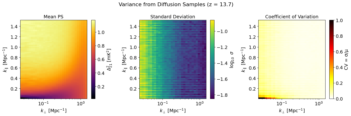
6. Uncertainty Quantification from Diffusion Samples
The diffusion model generates multiple samples for each input, allowing variance estimation.
[44]:
# Get the raw output which contains PS_2D_samples
ps_samples = ps_output.PS_2D_samples[:1]  # Shape: (1, n_z, n_samples, 32, 64)
print(f"PS samples shape: {ps_samples.shape}")

# Compute variance per pixel
ps_mean = np.mean(ps_samples, axis=2).value
ps_std = np.std(ps_samples, axis=2).value
ps_var = np.var(ps_samples, axis=2).value

print(f"PS mean shape: {ps_mean.shape}")
print(f"PS std shape: {ps_std.shape}")
PS samples shape: (1, 10, 100, 32, 64)
PS mean shape: (1, 10, 32, 64)
PS std shape: (1, 10, 32, 64)
[48]:
# Plot variance map for one redshift
z_idx = 5  # Use the same z_idx as the comparison plots

# Use emulator k-grids
kperp_emu = emu.properties.kperp
kpar_emu = emu.properties.kpar

fig, axes = plt.subplots(1, 3, figsize=(15, 5))

# Mean PS
im0 = axes[0].pcolormesh(kperp_emu, kpar_emu, ps_mean[0, z_idx].T, cmap='inferno')
axes[0].set_title('Mean PS', fontsize=14)
axes[0].set_xlabel(r'$k_\perp$ [Mpc$^{-1}$]')
axes[0].set_ylabel(r'$k_\parallel$ [Mpc$^{-1}$]')
axes[0].set_xscale('log')
plt.colorbar(im0, ax=axes[0], label=r'$\Delta^2_{21}$ [mK$^2$]')

# Standard deviation
im1 = axes[1].pcolormesh(kperp_emu, kpar_emu, np.log10(ps_std[0, z_idx] + 1e-10).T, cmap='viridis')
axes[1].set_title('Standard Deviation', fontsize=14)
axes[1].set_xlabel(r'$k_\perp$ [Mpc$^{-1}$]')
axes[1].set_ylabel(r'$k_\parallel$ [Mpc$^{-1}$]')
axes[1].set_xscale('log')
plt.colorbar(im1, ax=axes[1], label=r'$\log_{10}$ $\sigma$')

# Coefficient of variation (std/mean)
cv = ps_std[0, z_idx] / (ps_mean[0, z_idx] + 1e-10)
im2 = axes[2].pcolormesh(kperp_emu, kpar_emu, cv.T, cmap='hot_r', vmin=0, vmax=1)
axes[2].set_title('Coefficient of Variation', fontsize=14)
axes[2].set_xlabel(r'$k_\perp$ [Mpc$^{-1}$]')
axes[2].set_ylabel(r'$k_\parallel$ [Mpc$^{-1}$]')
axes[2].set_xscale('log')
plt.colorbar(im2, ax=axes[2], label='CV = σ/μ')

z_label = ps_redshifts[z_idx] if ps_redshifts is not None else z_idx
plt.suptitle(f'Variance from Diffusion Samples (z = {z_label:.1f})', fontsize=16)
plt.tight_layout()
plt.show()
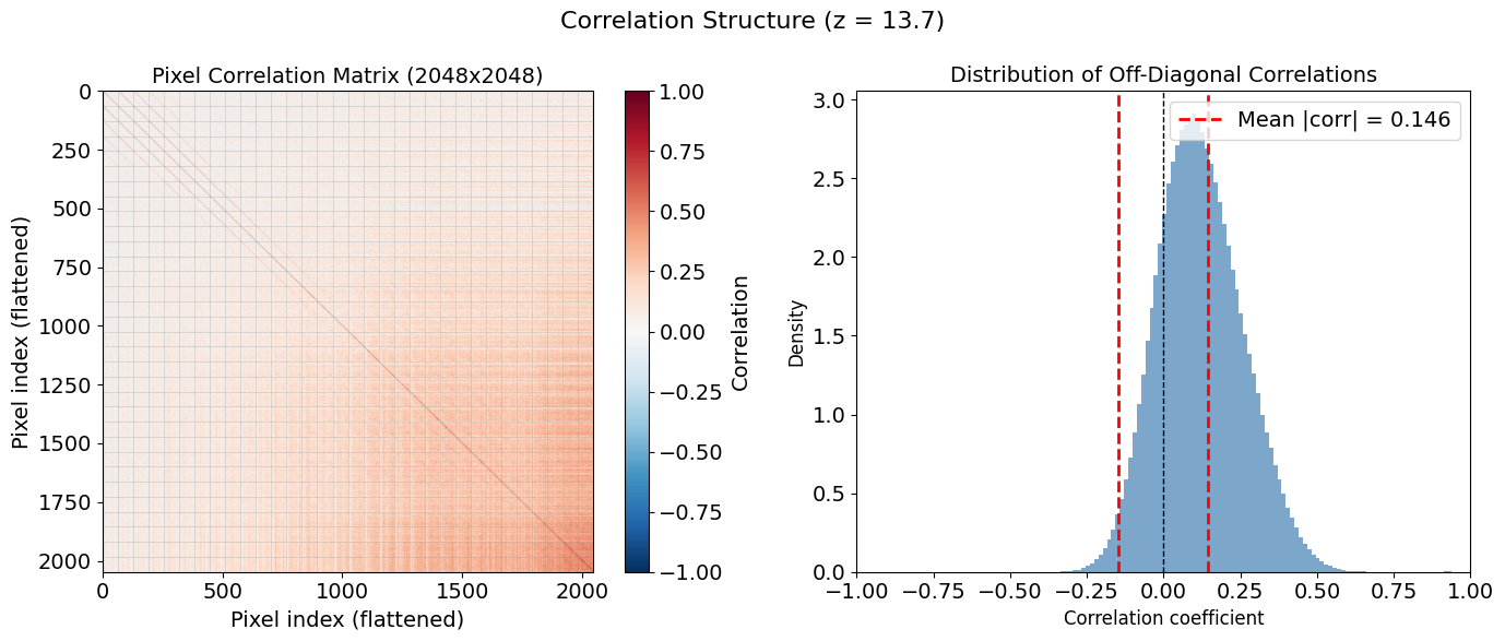
Covariance and Correlation Analysis
The diffusion model samples allow us to compute the full covariance matrix between all \((k_\perp, k_\parallel)\) pixels. This reveals the correlations induced by the diffusion process.
[51]:
# Compute full covariance matrix from samples
# Flatten samples to (n_samples, n_pixels)
H, W = ps_samples.shape[-2], ps_samples.shape[-1]
n_samples_cov = ps_samples.shape[2]
n_pixels = H * W

samples_flat = ps_samples[0, z_idx].reshape(n_samples_cov, -1).value  # (n_samples, H*W)

# Center the samples
samples_centered = samples_flat - samples_flat.mean(axis=0, keepdims=True)

# Compute covariance matrix: Cov[i,j] = E[(X_i - μ_i)(X_j - μ_j)]
cov_matrix = (samples_centered.T @ samples_centered) / (n_samples_cov - 1)
print(f"Covariance matrix shape: {cov_matrix.shape}")

# Compute correlation matrix from covariance
std_vec = np.sqrt(np.diag(cov_matrix))
std_outer = np.outer(std_vec, std_vec)
corr_matrix = cov_matrix / (std_outer + 1e-10)

# Clip correlation to [-1, 1] due to numerical precision
corr_matrix = np.clip(corr_matrix, -1, 1)
print(f"Correlation matrix shape: {corr_matrix.shape}")

# Compute diagnostic statistics
diag_var = np.diag(cov_matrix)
total_var = np.sum(diag_var)
off_diag_var = np.sum(np.abs(cov_matrix)) - total_var
diag_frac = total_var / (total_var + off_diag_var)

off_diag_mask = ~np.eye(n_pixels, dtype=bool)
mean_abs_corr = np.mean(np.abs(corr_matrix[off_diag_mask]))
max_abs_corr = np.max(np.abs(corr_matrix[off_diag_mask]))

z_label = ps_redshifts[z_idx] if ps_redshifts is not None else z_idx
print(f"\nCovariance diagnostics at z = {z_label:.1f}:")
print(f"  Diagonal fraction: {diag_frac:.3f}")
print(f"  Mean |off-diag correlation|: {mean_abs_corr:.3f}")
print(f"  Max |off-diag correlation|: {max_abs_corr:.3f}")
Covariance matrix shape: (2048, 2048)
Correlation matrix shape: (2048, 2048)

Covariance diagnostics at z = 13.7:
  Diagonal fraction: 0.007
  Mean |off-diag correlation|: 0.146
  Max |off-diag correlation|: 0.967
[52]:
# Plot correlation matrix
fig, axes = plt.subplots(1, 2, figsize=(14, 6))

# Full correlation matrix
im0 = axes[0].imshow(corr_matrix, cmap='RdBu_r', vmin=-1, vmax=1, aspect='auto')
axes[0].set_title(f'Pixel Correlation Matrix ({n_pixels}x{n_pixels})', fontsize=14)
axes[0].set_xlabel('Pixel index (flattened)')
axes[0].set_ylabel('Pixel index (flattened)')
plt.colorbar(im0, ax=axes[0], label='Correlation')

# Add grid lines to show 32x64 block structure
for i in range(0, n_pixels+1, W):
    axes[0].axhline(i-0.5, color='gray', alpha=0.3, lw=0.5)
    axes[0].axvline(i-0.5, color='gray', alpha=0.3, lw=0.5)

# Histogram of off-diagonal correlations
off_diag_corrs = corr_matrix[off_diag_mask]
axes[1].hist(off_diag_corrs, bins=100, alpha=0.7, density=True, color='steelblue')
axes[1].axvline(0, color='k', ls='--', lw=1)
axes[1].axvline(mean_abs_corr, color='r', ls='--', lw=2,
                label=f'Mean |corr| = {mean_abs_corr:.3f}')
axes[1].axvline(-mean_abs_corr, color='r', ls='--', lw=2)
axes[1].set_xlabel('Correlation coefficient', fontsize=12)
axes[1].set_ylabel('Density', fontsize=12)
axes[1].set_title('Distribution of Off-Diagonal Correlations', fontsize=14)
axes[1].legend(loc='upper right')
axes[1].set_xlim(-1, 1)

z_label = ps_redshifts[z_idx] if ps_redshifts is not None else z_idx
plt.suptitle(f'Correlation Structure (z = {z_label:.1f})', fontsize=16)
plt.tight_layout()
plt.show()
[53]:
# Spatial correlation maps: correlation of each pixel with reference pixels
kperp_emu = emu.properties.kperp
kpar_emu = emu.properties.kpar

# Define reference pixels: center and corner
center_idx = (H // 2) * W + (W // 2)  # Center pixel
corner_idx = 0  # Top-left corner
mid_k_idx = (H // 4) * W + (W // 2)  # Mid-k region

# Extract correlation with reference pixels and reshape to 2D
corr_with_center = corr_matrix[center_idx, :].reshape(H, W)
corr_with_corner = corr_matrix[corner_idx, :].reshape(H, W)
corr_with_mid = corr_matrix[mid_k_idx, :].reshape(H, W)

fig, axes = plt.subplots(1, 3, figsize=(16, 5))

# Correlation with center pixel
im0 = axes[0].pcolormesh(kperp_emu, kpar_emu, corr_with_center.T,
                          cmap='RdBu_r', vmin=-1, vmax=1)
axes[0].plot(kperp_emu[H//2], kpar_emu[W//2], 'k*', ms=15, label='Reference')
axes[0].set_title('Correlation with Center Pixel', fontsize=14)
axes[0].set_xlabel(r'$k_\perp$ [Mpc$^{-1}$]')
axes[0].set_ylabel(r'$k_\parallel$ [Mpc$^{-1}$]')
axes[0].set_xscale('log')
axes[0].legend()
plt.colorbar(im0, ax=axes[0], label='Correlation')

# Correlation with corner pixel (low-k)
im1 = axes[1].pcolormesh(kperp_emu, kpar_emu, corr_with_corner.T,
                          cmap='RdBu_r', vmin=-1, vmax=1)
axes[1].plot(kperp_emu[0], kpar_emu[0], 'k*', ms=15, label='Reference')
axes[1].set_title('Correlation with Low-k Corner', fontsize=14)
axes[1].set_xlabel(r'$k_\perp$ [Mpc$^{-1}$]')
axes[1].set_ylabel(r'$k_\parallel$ [Mpc$^{-1}$]')
axes[1].set_xscale('log')
axes[1].legend()
plt.colorbar(im1, ax=axes[1], label='Correlation')

# Correlation with mid-k pixel
im2 = axes[2].pcolormesh(kperp_emu, kpar_emu, corr_with_mid.T,
                          cmap='RdBu_r', vmin=-1, vmax=1)
axes[2].plot(kperp_emu[H//4], kpar_emu[W//2], 'k*', ms=15, label='Reference')
axes[2].set_title('Correlation with Mid-k Pixel', fontsize=14)
axes[2].set_xlabel(r'$k_\perp$ [Mpc$^{-1}$]')
axes[2].set_ylabel(r'$k_\parallel$ [Mpc$^{-1}$]')
axes[2].set_xscale('log')
axes[2].legend()
plt.colorbar(im2, ax=axes[2], label='Correlation')

z_label = ps_redshifts[z_idx] if ps_redshifts is not None else z_idx
plt.suptitle(f'Spatial Correlation Maps (z = {z_label:.1f})', fontsize=16)
plt.tight_layout()
plt.show()

print("\nCorrelation length analysis:")
print(f"  Center pixel self-correlation: {corr_with_center[H//2, W//2]:.3f}")
print(f"  Center-corner correlation: {corr_with_center[0, 0]:.3f}")
print(f"  This indicates {'strong' if abs(corr_with_center[0, 0]) > 0.3 else 'weak'} "
      f"long-range correlations in the diffusion samples.")
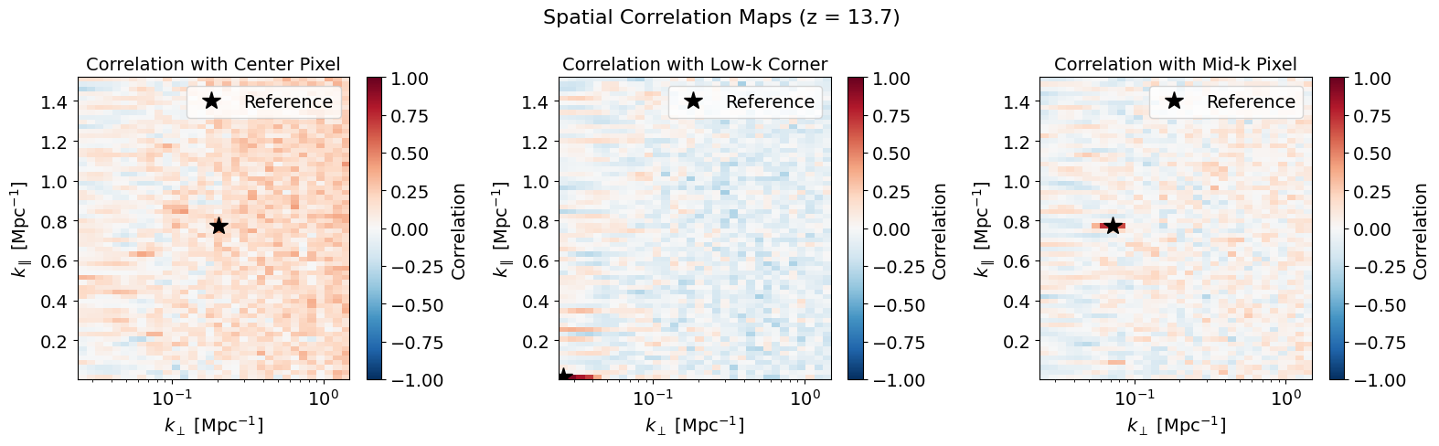
Correlation length analysis:
  Center pixel self-correlation: 1.000
  Center-corner correlation: 0.024
  This indicates weak long-range correlations in the diffusion samples.
7. Comparison: EM vs ODE Sampling
The diffusion model supports two sampling methods:
Euler-Maruyama (EM): Stochastic sampling, faster, allows variance estimation
Probability-flow ODE: Deterministic sampling, slower but exact likelihood
[ ]:
import time

# Single parameter for comparison
test_single = ps_test_params[:1]

# EM sampling
t0 = time.time()
_, out_em, _ = emu.predict(test_single, ps_2d_redshifts=ps_redshifts,
                           ps_sampling_method='em', n_realisations=50, verbose=False)
t_em = time.time() - t0

# ODE sampling
t0 = time.time()
_, out_ode, _ = emu.predict(test_single, ps_2d_redshifts=ps_redshifts,
                            ps_sampling_method='ode', n_realisations=50, verbose=False)
t_ode = time.time() - t0

print(f"EM sampling:  {t_em:.2f}s")
print(f"ODE sampling: {t_ode:.2f}s")
[ ]:
# Compare EM vs ODE - use same z_idx as before
z_idx_compare = 5  # Should match the subset of redshifts we selected

ps_em = out_em['PS_2D'][0, z_idx_compare]
ps_ode = out_ode['PS_2D'][0, z_idx_compare]

fig, axes = plt.subplots(1, 3, figsize=(15, 5))

vmin = min(np.log10(ps_em).min(), np.log10(ps_ode).min())
vmax = max(np.log10(ps_em).max(), np.log10(ps_ode).max())

kperp_emu = emu.properties.kperp
kpar_emu = emu.properties.kpar

im0 = axes[0].pcolormesh(kperp_emu, kpar_emu, np.log10(ps_em).T,
                          vmin=vmin, vmax=vmax, cmap='inferno')
axes[0].set_title(f'EM Sampling ({t_em:.1f}s)', fontsize=14)
axes[0].set_xlabel(r'$k_\perp$ [Mpc$^{-1}$]')
axes[0].set_ylabel(r'$k_\parallel$ [Mpc$^{-1}$]')
axes[0].set_xscale('log')
plt.colorbar(im0, ax=axes[0], label=r'$\log_{10}$ PS')

im1 = axes[1].pcolormesh(kperp_emu, kpar_emu, np.log10(ps_ode).T,
                          vmin=vmin, vmax=vmax, cmap='inferno')
axes[1].set_title(f'ODE Sampling ({t_ode:.1f}s)', fontsize=14)
axes[1].set_xlabel(r'$k_\perp$ [Mpc$^{-1}$]')
axes[1].set_ylabel(r'$k_\parallel$ [Mpc$^{-1}$]')
axes[1].set_xscale('log')
plt.colorbar(im1, ax=axes[1], label=r'$\log_{10}$ PS')

# Difference
diff = np.log10(ps_em) - np.log10(ps_ode)
vlim = np.percentile(np.abs(diff), 95)
im2 = axes[2].pcolormesh(kperp_emu, kpar_emu, diff.T,
                          vmin=-vlim, vmax=vlim, cmap='RdBu_r')
axes[2].set_title(f'EM - ODE (RMS: {np.sqrt(np.mean(diff**2)):.3f})', fontsize=14)
axes[2].set_xlabel(r'$k_\perp$ [Mpc$^{-1}$]')
axes[2].set_ylabel(r'$k_\parallel$ [Mpc$^{-1}$]')
axes[2].set_xscale('log')
plt.colorbar(im2, ax=axes[2], label=r'$\Delta \log_{10}$ PS')

z_label = ps_redshifts[z_idx_compare] if ps_redshifts is not None else z_idx_compare
plt.suptitle(f'EM vs ODE Sampling Comparison (z = {z_label:.1f})', fontsize=16)
plt.tight_layout()
plt.show()
Using the MHEmulatorErrors Class
The MH (v3) emulator provides error statistics via the MHEmulatorErrors class, which differs significantly from ACG/Radio emulators:
Key Differences:
Absolute errors in physical units (not fractional %)
Output-dependent errors: computed from
FE% × |output_value|2D PS error statistics: variance, covariance, and correlation matrices
Sampling method support: different errors for ‘em’ vs ‘ode’ sampling
[ ]:
# Get the error object from the prediction
_, output_single, errors = emu.predict(test_params[0:1], verbose=False)

# Inspect the error object
print(f"Error type: {type(errors).__name__}")
print(f"\nAvailable error fields: {errors.keys()}")
print(f"\nError summary:\n{errors.summary()}")
Absolute Errors with Physical Units
Unlike ACG/Radio which store FE%, MHEmulatorErrors provides absolute errors with proper astropy units. For log-space quantities (PS, UVLFs), errors are in dex (log10 units).
[ ]:
# Check units of each error field
print("Error field units:")
print(f"  PS_err: {errors.PS_err.unit} (dex - error on log10 PS)")
print(f"  Tb_err: {errors.Tb_err.unit} (absolute mK error)")
print(f"  xHI_err: {errors.xHI_err.unit} (absolute neutral fraction error)")
print(f"  Ts_err: {errors.Ts_err.unit} (absolute K error)")
print(f"  tau_err: {errors.tau_err.unit} (absolute optical depth error)")
print(f"  UVLFs_logerr: {errors.UVLFs_logerr.unit} (dex - error on log10 LF)")

# Median PS error interpretation
median_ps_err = np.nanmedian(errors.PS_err.value)
print(f"\nMedian PS error: {median_ps_err:.3f} dex")
print(f"  This means log10(PS) predictions are typically off by ~{median_ps_err:.3f}")
print(f"  In linear PS, this is a factor of 10^{median_ps_err:.3f} ≈ {10**median_ps_err:.2f} ({(10**median_ps_err - 1)*100:.0f}% error)")
2D Power Spectrum Error Statistics (Unique to MH Emulator)
The MH emulator’s diffusion model provides advanced error statistics for the 2D power spectrum:
Variance: Per-bin error variance from test set residuals
Covariance: Full covariance matrix between (kperp, kpar) bins
Correlation diagnostics:
ps_diagonal_fraction,ps_mean_abs_correlation
[ ]:
# Access 2D PS error statistics via the errors object
ps_var = errors.get_ps_variance()
ps_cov = errors.get_ps_covariance()

if ps_var is not None:
    print(f"2D PS variance shape: {ps_var.shape}")
    print(f"2D PS covariance shape: {ps_cov.shape if ps_cov is not None else 'N/A'}")
    print("\nCorrelation diagnostics:")
    print(f"  Diagonal fraction: {errors.ps_diagonal_fraction:.2%}")
    print("  (1.0 = uncorrelated errors, <1.0 = some correlation)")
    print(f"  Mean |off-diag correlation|: {errors.ps_mean_abs_correlation:.3f}")
    print("  (0 = uncorrelated, 1 = perfectly correlated)")
else:
    print("2D PS statistics not available (emulator loaded without 2D PS)")
[ ]:
# Visualize 2D PS variance and correlation matrix
if ps_var is not None and ps_cov is not None:
    fig, axes = plt.subplots(1, 3, figsize=(16, 5))

    # Get k-grids from emulator properties
    kperp = emu.properties.kperp
    kpar = emu.properties.kpar

    # Plot variance map
    im0 = axes[0].pcolormesh(kperp, kpar, ps_var.T, cmap='viridis')
    axes[0].set_xlabel(r'$k_\perp$ [Mpc$^{-1}$]')
    axes[0].set_ylabel(r'$k_\parallel$ [Mpc$^{-1}$]')
    axes[0].set_xscale('log')
    axes[0].set_title('2D PS Error Variance (FE%²)')
    plt.colorbar(im0, ax=axes[0], label='Variance')

    # Plot covariance matrix (subsampled for visibility)
    step = 8  # Subsample for clearer visualization
    cov_sub = ps_cov[::step, ::step]
    im1 = axes[1].imshow(cov_sub, cmap='RdBu_r', aspect='equal',
                         vmin=-np.percentile(np.abs(cov_sub), 95),
                         vmax=np.percentile(np.abs(cov_sub), 95))
    axes[1].set_title(f'Covariance Matrix (subsampled {step}x)')
    axes[1].set_xlabel('Pixel index')
    axes[1].set_ylabel('Pixel index')
    plt.colorbar(im1, ax=axes[1], label='Covariance')

    # Compute and plot correlation matrix
    std = np.sqrt(np.diag(ps_cov))
    std_outer = np.outer(std, std)
    corr = ps_cov / std_outer
    corr_sub = corr[::step, ::step]

    im2 = axes[2].imshow(corr_sub, cmap='RdBu_r', aspect='equal', vmin=-1, vmax=1)
    axes[2].set_title('Correlation Matrix (subsampled)')
    axes[2].set_xlabel('Pixel index')
    axes[2].set_ylabel('Pixel index')
    plt.colorbar(im2, ax=axes[2], label='Correlation')

    plt.suptitle('MH Emulator: 2D PS Error Statistics', fontsize=14, y=1.02)
    plt.tight_layout()
    plt.show()
else:
    print("Load emulator with emulate_2d_ps=True to access these statistics")
Summary
This tutorial demonstrated the v3 (MH) emulator capabilities:
1D Summaries: Global \(T_b\), \(x_{\mathrm{HI}}\), \(T_s\), UVLFs, and \(\tau_e\) emulated by LSTM networks
2D Power Spectrum: \(P(k_\perp, k_\parallel)\) emulated by a score-based diffusion model
Uncertainty Quantification:
Variance/standard deviation maps from diffusion samples
Full covariance matrix computation between PS pixels
Correlation structure analysis and spatial correlation maps
Sampling Methods: EM (fast, stochastic) vs ODE (slower, deterministic)
The emulator achieves:
Sub-percent median fractional errors on most 1D summaries
~10% median FE on 2D PS for most k-modes
Full probabilistic uncertainty through diffusion sampling
Pixel-by-pixel covariance for downstream statistical analyses