21cmEMUv2: Adding Radio Background

In this tutorial we demonstrate how to use the emulator that was trained on a 21cmFAST model which includes a radio background (see Cang+24 for more details).

import matplotlib.patches as mpatches
import matplotlib.pyplot as plt
import numpy as np
from matplotlib import rcParams

rcParams.update({"font.size": 12})

from corner import corner

from py21cmemu import Emulator

We begin by loading a database of summaries to use as examples in this tutorial.

This database is a fraction of the test set of the emulator.

with np.load("Radio_Test_data_sample.npz") as f:
    test_params = f["params"]
    test_Tb = f["Tb"]
    test_Tr = f["Tr"]
    test_PS = f["PS"]
    test_xHI = f["xHI"]
    test_tau = f["tau"]
    PS_k = f["PS_k"]
    PS_z = f["PS_z"]
    test_z = f["redshifts"]
    zs = f["redshifts"]

To load the radio emulator, we just need to specify emulator="radio_background" when initialising the Emulator class.

If no emulator is specified, then the default emulator is loaded.

emu = Emulator(emulator="radio_background")

After initialising the Emulator class correctly, the rest of the calls are exactly the same as for the default emulator:

normed_input_params, output, output_errors = emu.predict(test_params)

The outputs can be accessed in the same way as for the default emulator:

print("Summaries returned by the radio_background emulator are: ", list(output.keys()))
print(
    "Shape of radio background temperature summary output: [Nsamples, N redshift bins] = ",
    output.Tr.shape,
)

Summaries returned by the radio_background emulator are:  ['Tb', 'xHI', 'Tr', 'PS', 'tau']
Shape of radio background temperature summary output: [Nsamples, N redshift bins] =  (1000, 103)

You can inspect which parameters must be supplied in log10 space using LOG_PARAMETERS, and the full parameter list with units via PARAMETERS:

from py21cmemu.inputs import RadioEmulatorInput

radio_in = RadioEmulatorInput()

print("All parameters and their units:")
for name, unit in radio_in.PARAMETERS.items():
    marker = " ← log10 input required" if name in radio_in.LOG_PARAMETERS else ""
    print(f"  {name:15s}  [{unit}]{marker}")

# The test parameters are already in the correct physical space:
# fR_mini, L_X_MINI, F_STAR7_MINI, F_ESC7_MINI are in log10 space
# A_LW is linear
print("Test parameter column order:", radio_in.astro_param_keys)
print("First test param:", test_params[0])

You can also normalize/un-normalize parameters using RadioEmulatorInput.normalize() and undo_normalization(), which map physical parameters to the internal [0, 1] range used by the emulator. This is useful if you want to inspect the normalized parameter space.

# Normalize physical params to [0,1] internal range
normed_params = radio_in.normalize(test_params)
print(
    "Normalized param range (should be [0,1]):",
    normed_params.min().round(3),
    "–",
    normed_params.max().round(3),
)

# Recover physical params from normalized (round-trip check)
recovered = radio_in.undo_normalization(normed_params)
print("Round-trip recovery max abs error:", np.abs(recovered - test_params).max())

True

Let’s make some plots to compare them.

We start by defining a function to calculate the fractional error (FE).

# Calculate fractional error (FE)
def print_fe(pred, true, name="", ret=False, floor=None):
    if floor is not None:
        m = abs(true) < floor
        true_final = true.copy()
        true_final[m] = floor
    else:
        true_final = true

    frac_err = abs((pred - true) / true_final) * 100.0
    print(
        "FE (%) "
        + name
        + ": Median: %.4f, 68%%CI: %.4f, 95%%CI: %.4f"
        % tuple(np.nanpercentile(frac_err, [50, 84, 97.5]))
    )
    print(
        "Abs diff "
        + name
        + ": Median: %.5f, 68%%CI: %.5f, 95%%CI: %.5f"
        % tuple(np.nanpercentile(abs(pred - true), [50, 84, 97.5]))
    )

    print("FE " + name + " STD: %.3f" % np.nanstd(frac_err))
    if ret:
        return frac_err

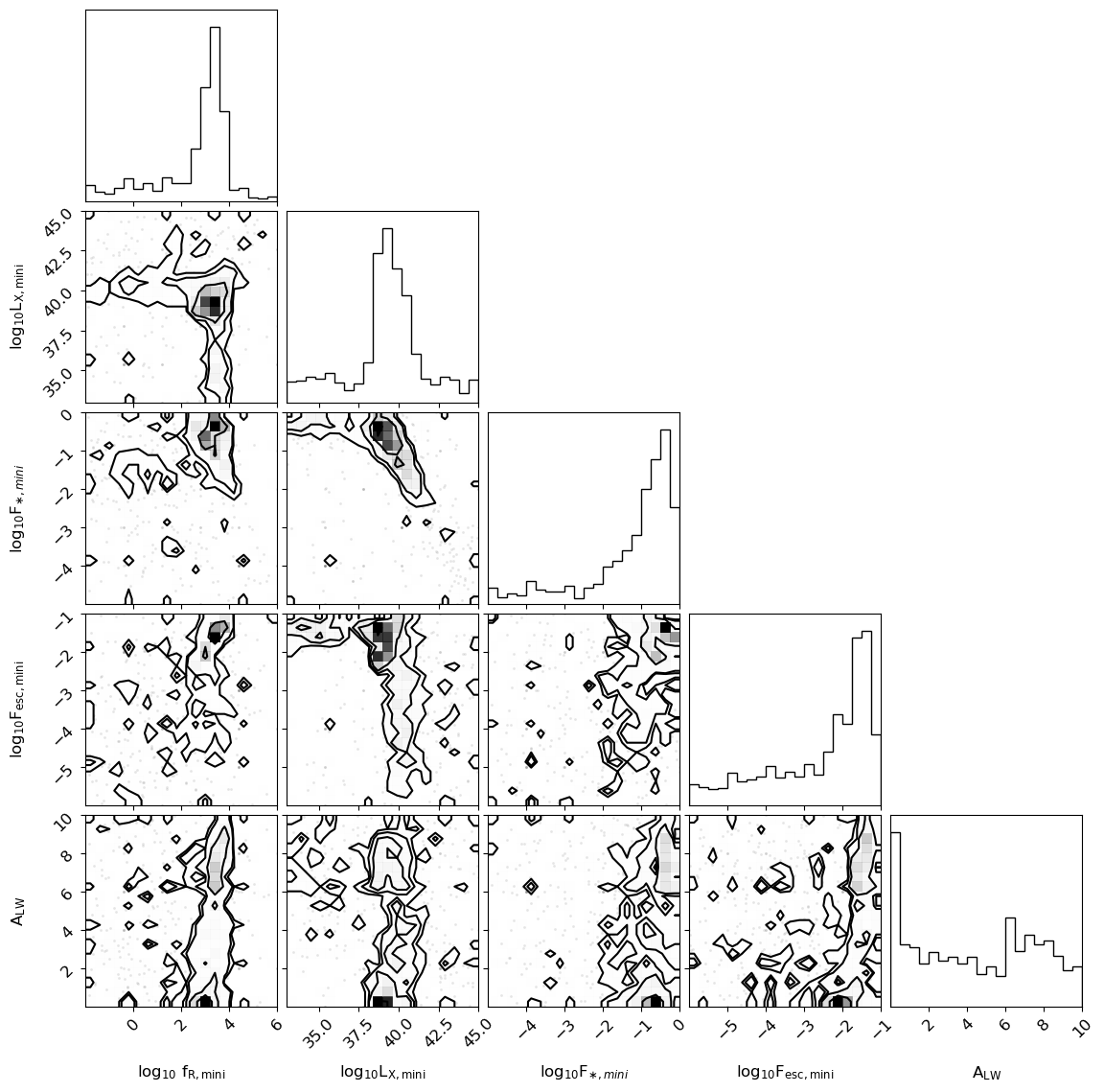
First, we can look at the parameter distribution of the test set sample provided:

labels = output.properties.parameter_labels
corner(test_params, labels=labels)
plt.show()

Next, we can calculate the emulator performance (fractional error) on each summary and display the median, 68%, and 95% confidence limits:

# print performance
Tb_frac_err = print_fe(output.Tb.value, test_Tb, name="Tb", ret=True, floor=5)

FE (%) Tb: Median: 2.4298, 68%CI: 9.1370, 95%CI: 29.9726
Abs diff Tb: Median: 0.46664, 68%CI: 3.01442, 95%CI: 14.78150
FE Tb STD: 11.082

Tr_frac_err = print_fe(output.Tr.value, test_Tr, name="Tr", ret=True, floor=1e-4)

FE (%) Tr: Median: 1.3364, 68%CI: 4.7003, 95%CI: 99.9828
Abs diff Tr: Median: 0.79453, 68%CI: 9.19828, 95%CI: 35.84473
FE Tr STD: 22.876

xHI_frac_err = print_fe(output.xHI.value, test_xHI, name="xHI", ret=True, floor=1e-3)

FE (%) xHI: Median: 0.1890, 68%CI: 11.3611, 95%CI: 71.3078
Abs diff xHI: Median: 0.00030, 68%CI: 0.00162, 95%CI: 0.00793
FE xHI STD: 67.385

PS_frac_err = print_fe(output.PS.value, test_PS, name="PS", ret=True, floor=1e-2)

FE (%) PS: Median: 3.4283, 68%CI: 17.7266, 95%CI: 69.1445
Abs diff PS: Median: 0.03751, 68%CI: 27.25376, 95%CI: 6927.05156
FE PS STD: 59.203

tau_frac_err = print_fe(output.tau.value, test_tau, name="tau", ret=True)

FE (%) tau: Median: 0.2742, 68%CI: 0.7194, 95%CI: 1.6971
Abs diff tau: Median: 0.00032, 68%CI: 0.00085, 95%CI: 0.00211
FE tau STD: 0.526

We calculate the absolute errors of each summary for the plots:

xHI_diff = abs(output.xHI.value - test_xHI)
diff_err_xHI_z = np.nanpercentile(xHI_diff, [2.5, 16, 50, 84, 97.5], axis=0)

PS_diff = abs(output.PS.value - test_PS)
diff_err_PS_z = np.nanpercentile(PS_diff, [2.5, 16, 50, 84, 97.5], axis=0)

Tb_diff = abs(output.Tb.value - test_Tb)
diff_err_Tb_z = np.nanpercentile(Tb_diff, [2.5, 16, 50, 84, 97.5], axis=0)

Tr_diff = abs(output.Tr.value - test_Tr)
diff_err_Tr_z = np.nanpercentile(Tr_diff, [2.5, 16, 50, 84, 97.5], axis=0)

tau_diff = abs(output.tau.value - test_tau)

Let’s shuffle the parameters and plot N = 10 examples at a time.

The seed is set to 42 for reproducibility.

idxs = np.arange(test_tau.shape[0])
np.random.seed(42)
np.random.shuffle(idxs)

N = 10
idxs = idxs[:N]

cs = ["r", "g", "b", "lime", "cyan", "orange", "k", "tan", "firebrick", "magenta"]

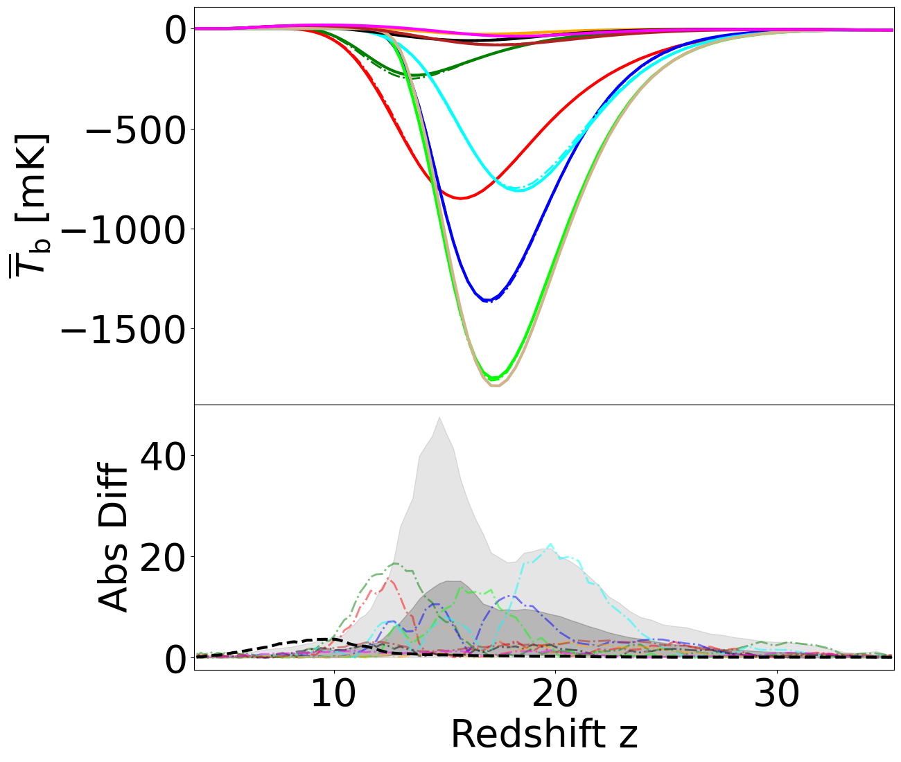
rcParams.update({"font.size": 40})

fig, axs = plt.subplots(
    nrows=2,
    ncols=1,
    sharex=True,
    figsize=(14, 12),
    gridspec_kw=dict(height_ratios=[3, 2], hspace=0),
)
axs = axs.flatten()

# inset axes...
# axins = axs[1].inset_axes([0.35, 0.2, 0.6, 0.47])

for i, c in zip(idxs, cs, strict=False):
    if i == N - 1:
        labels = ["21cmEMU", "Test Set"]
    else:
        labels = [None, None]
    axs[0].plot(zs, test_Tb[i, :], lw=3, color=c, label=labels[1])
    axs[1].plot(zs, Tb_diff[i, :], ls="-.", alpha=0.5, lw=2, color=c)
    axs[0].plot(zs, output.Tb[i, :].value, lw=2, ls="-.", color=c, label=labels[0])

axs[1].plot(zs, diff_err_Tb_z[2, :][::-1], ls="--", lw=3, color="k", label=r"Median")
axs[1].fill_between(
    zs, diff_err_Tb_z[1, :], diff_err_Tb_z[3, :], color="k", alpha=0.2, label=r"68% CI"
)
axs[1].fill_between(
    zs, diff_err_Tb_z[0, :], diff_err_Tb_z[4, :], color="k", alpha=0.1, label=r"95% CI"
)


axs[0].set_ylabel(r"$\overline{T}_{\rm{b}}$ [mK]")
axs[1].set_ylabel(r"Abs Diff")
axs[1].set_xlabel(r"Redshift z")
axs[1].tick_params(axis="both", which="major")
axs[1].tick_params(axis="both", which="minor")
axs[0].tick_params(axis="y", which="major")
axs[0].tick_params(axis="y", which="minor")
axs[0].set_xlim(zs[0] - 0.1, zs[-1] + 0.1)

plt.tight_layout()
plt.show()

rcParams.update({"font.size": 40})

fig, axs = plt.subplots(
    nrows=2,
    ncols=1,
    sharex=True,
    figsize=(14, 12),
    gridspec_kw=dict(height_ratios=[3, 2], hspace=0),
)
axs = axs.flatten()

for i, c in zip(idxs, cs, strict=False):
    if i == N - 1:
        labels = ["21cmEMU", "Test Set"]
    else:
        labels = [None, None]
    axs[0].plot(zs, test_Tr[i, :], lw=3, color=c, label=labels[1])
    axs[1].plot(zs, Tr_diff[i, :], ls="-.", alpha=0.5, lw=2, color=c)
    axs[0].plot(zs, output.Tr[i, :].value, lw=2, ls="-.", color=c, label=labels[0])

axs[1].plot(zs[::-1], diff_err_Tr_z[2, :], ls="--", lw=3, color="k", label=r"Median")
axs[1].fill_between(
    zs,
    diff_err_Tr_z[1, :],
    diff_err_Tr_z[3, :][::-1],
    color="k",
    alpha=0.2,
    label=r"68% CI",
)
axs[1].fill_between(
    zs,
    diff_err_Tr_z[0, :],
    diff_err_Tr_z[4, :][::-1],
    color="k",
    alpha=0.1,
    label=r"95% CI",
)


axs[0].set_ylabel(r"$\overline{T}_{\rm{r}}$ [K]")
axs[1].set_ylabel(r"Abs Diff")
axs[1].set_xlabel(r"Redshift z")
axs[1].tick_params(axis="both", which="major")
axs[1].tick_params(axis="both", which="minor")
axs[0].tick_params(axis="y", which="major")
axs[0].tick_params(axis="y", which="minor")
axs[0].set_xlim(zs[0] - 0.1, zs[-1] + 0.1)
axs[0].set_yscale("log")
axs[1].set_yscale("log")

plt.tight_layout()
plt.show()

As you can see, for the radio background temperature, the emulator output wiggles around the correct value.

This behaviour is known. However, it wouldn’t significantly affect the result of an inference (as it does not bias the result in any way).

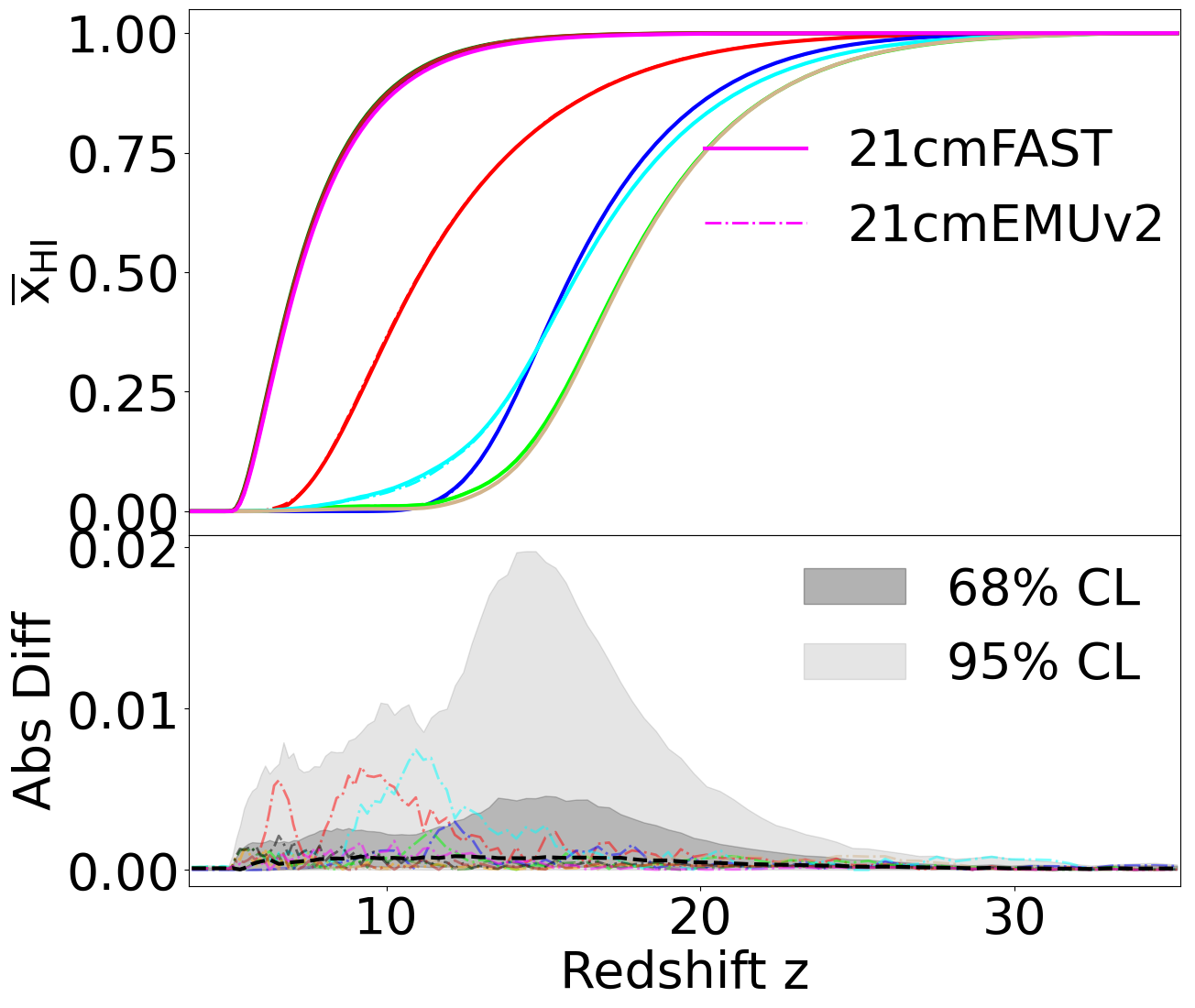
rcParams.update({"font.size": 40})

fig, axs = plt.subplots(
    nrows=2,
    ncols=1,
    sharex=True,
    figsize=(14, 12),
    gridspec_kw=dict(height_ratios=[3, 2], hspace=0),
)
axs = axs.flatten()

# inset axes...
# axins = axs[1].inset_axes([0.35, 0.2, 0.6, 0.47])

for i, c, num in zip(idxs, cs, range(N), strict=False):
    if num == N - 1:
        labels = ["21cmEMUv2", "21cmFAST"]
    else:
        labels = [None, None]
    axs[0].plot(zs, test_xHI[i, :], lw=3, color=c, label=labels[1])
    axs[1].plot(zs, xHI_diff[i, :], ls="-.", alpha=0.5, lw=2, color=c)
    axs[0].plot(zs, output.xHI[i, :].value, lw=2, ls="-.", color=c, label=labels[0])

axs[0].legend(loc=(0.5, 0.5), frameon=False)  # framealpha=0.3)
axs[1].plot(zs, diff_err_xHI_z[2, :], ls="--", lw=3, color="k", label=r"Median")
axs[1].fill_between(
    zs,
    diff_err_xHI_z[1, :],
    diff_err_xHI_z[3, :],
    color="k",
    alpha=0.2,
    label=r"68% CI",
)
axs[1].fill_between(
    zs,
    diff_err_xHI_z[0, :],
    diff_err_xHI_z[4, :],
    color="k",
    alpha=0.1,
    label=r"95% CI",
)

handles = [
    mpatches.Patch(color="k", label="68% CL", alpha=0.3),
    mpatches.Patch(color="k", label="95% CL", alpha=0.1),
]
plt.legend(handles=handles, loc=(0.6, 0.5), frameon=False)
axs[0].set_ylabel(r"$\overline{\mathrm{x}}_{\rm{HI}}$")
axs[1].set_ylabel(r"Abs Diff")
axs[1].set_xlabel(r"Redshift z")

plt.xlim(zs[0] - 0.1, zs[-1] + 0.1)

plt.tight_layout()
plt.show()

We plot the redshift evolution of the 21-cm power spectrum around scales \(k \sim 0.1 \rm{Mpc}^{-1}\):

kbin = 11
PS_k[kbin]

0.10969735366408447

rcParams.update({"font.size": 40})

fig, axs = plt.subplots(
    nrows=2,
    ncols=1,
    sharex=True,
    figsize=(14, 12),
    gridspec_kw=dict(height_ratios=[3, 2], hspace=0),
)
axs = axs.flatten()


for i, c, num in zip(idxs, cs, range(N), strict=False):
    if num == N - 1:
        labels = ["21cmEMUv2", "21cmFAST"]
    else:
        labels = [None, None]
    axs[0].plot(PS_z, test_PS[i, :, kbin], lw=3, color=c, label=labels[1])
    axs[1].plot(PS_z, PS_diff[i, :, kbin], ls="-.", alpha=0.5, lw=2, color=c)
    axs[0].plot(
        PS_z, output.PS[i, :, kbin].value, lw=2, ls="-.", color=c, label=labels[0]
    )

axs[0].legend(loc=(0.25, 0.01), frameon=False)  # framealpha=0.3)
axs[1].plot(PS_z, diff_err_PS_z[2, :, kbin], ls="--", lw=3, color="k", label=r"Median")
axs[1].fill_between(
    PS_z,
    diff_err_PS_z[1, :, kbin],
    diff_err_PS_z[3, :, kbin],
    color="k",
    alpha=0.2,
    label=r"68% CI",
)
axs[1].fill_between(
    PS_z,
    diff_err_PS_z[0, :, kbin],
    diff_err_PS_z[4, :, kbin],
    color="k",
    alpha=0.1,
    label=r"95% CI",
)

handles = [
    mpatches.Patch(color="k", label="68% CL", alpha=0.3),
    mpatches.Patch(color="k", label="95% CL", alpha=0.1),
]
plt.legend(handles=handles, loc=(0.6, 0.01), frameon=False)
axs[0].set_ylabel(r"$\Delta_{21}^2$ [mK$^2$]")
axs[1].set_ylabel(r"Abs Diff")
axs[1].set_xlabel(r"Redshift z")

axs[0].set_yscale("log")
axs[1].set_yscale("log")

plt.xlim(PS_z[0] - 0.1, PS_z[-1] + 0.1)

plt.tight_layout()
plt.show()

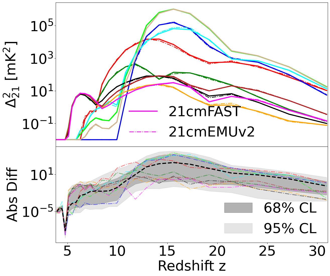
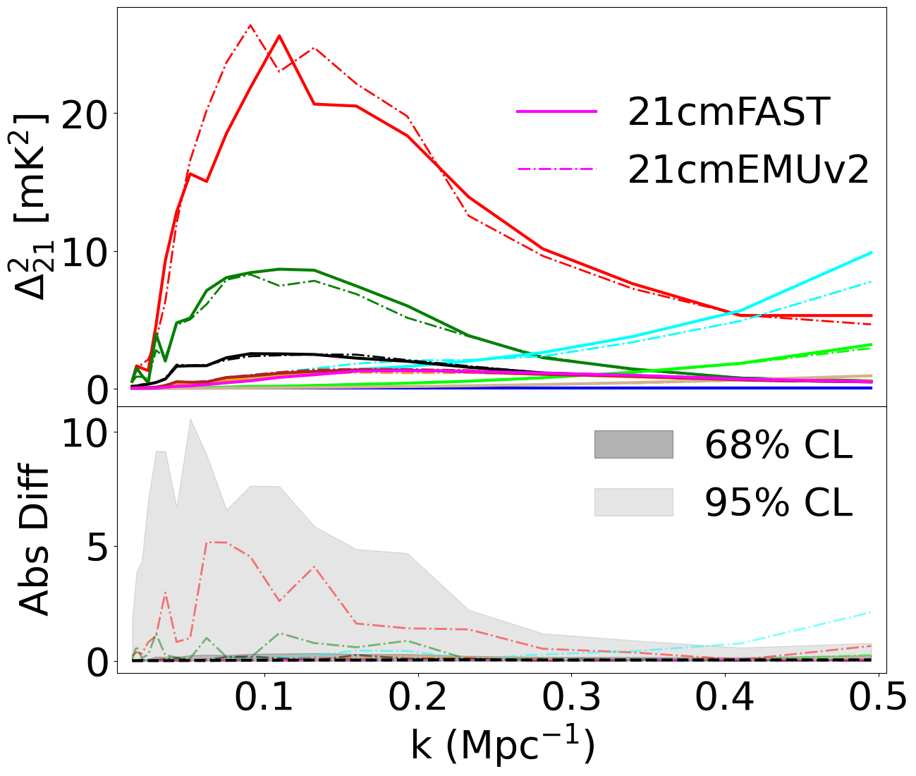
Now we plot the 21-cm power spectrum evolution at a fixed redshift of about \(z \sim 8.5\).

zbin = 11
PS_z[zbin]

8.46594037485638

rcParams.update({"font.size": 40})

fig, axs = plt.subplots(
    nrows=2,
    ncols=1,
    sharex=True,
    figsize=(14, 12),
    gridspec_kw=dict(height_ratios=[3, 2], hspace=0),
)
axs = axs.flatten()

for i, c, num in zip(idxs, cs, range(N), strict=False):
    if num == N - 1:
        labels = ["21cmEMUv2", "21cmFAST"]
    else:
        labels = [None, None]
    axs[0].plot(PS_k, test_PS[i, zbin, :], lw=3, color=c, label=labels[1])
    axs[1].plot(PS_k, PS_diff[i, zbin, :], ls="-.", alpha=0.5, lw=2, color=c)
    axs[0].plot(
        PS_k, output.PS[i, zbin, :].value, lw=2, ls="-.", color=c, label=labels[0]
    )

axs[0].legend(loc=(0.5, 0.5), frameon=False)  # framealpha=0.3)
axs[1].plot(PS_k, diff_err_PS_z[2, zbin, :], ls="--", lw=3, color="k", label=r"Median")
axs[1].fill_between(
    PS_k,
    diff_err_PS_z[1, zbin, :],
    diff_err_PS_z[3, zbin, :],
    color="k",
    alpha=0.2,
    label=r"68% CI",
)
axs[1].fill_between(
    PS_k,
    diff_err_PS_z[0, zbin, :],
    diff_err_PS_z[4, zbin, :],
    color="k",
    alpha=0.1,
    label=r"95% CI",
)

handles = [
    mpatches.Patch(color="k", label="68% CL", alpha=0.3),
    mpatches.Patch(color="k", label="95% CL", alpha=0.1),
]
plt.legend(handles=handles, loc=(0.6, 0.5), frameon=False)
axs[0].set_ylabel(r"$\Delta_{21}^2$ [mK$^2$]")
axs[1].set_ylabel(r"Abs Diff")
axs[1].set_xlabel(r"k (Mpc$^{-1}$)")

plt.xlim(PS_k[0] - 1e-2, PS_k[-1] + 1e-2)

plt.tight_layout()
plt.show()

tau_bins = np.linspace(min(test_tau), np.percentile(test_tau, 99.0), 15)
tau_binned_fe = np.zeros(len(tau_bins))
tau_binned_fe_68 = np.zeros((len(tau_bins), 2))
tau_binned_fe_95 = np.zeros((len(tau_bins), 2))

for i in range(len(tau_bins) - 1):
    mask = np.logical_and(test_tau >= tau_bins[i], test_tau < tau_bins[i + 1])
    low1, low, med, high, high1 = np.nanpercentile(
        tau_frac_err[mask], [2.5, 16, 50, 84, 97.5]
    )
    tau_binned_fe[i] = med
    tau_binned_fe_68[i, :] = [low, high]
    tau_binned_fe_95[i, :] = [low1, high1]

plt.figure(figsize=(10, 7))
rcParams.update({"font.size": 30})
plt.plot(tau_bins, tau_binned_fe, color="k", lw=2, ls="--")
plt.fill_between(
    tau_bins, tau_binned_fe_68[:, 0], tau_binned_fe_68[:, 1], color="k", alpha=0.2
)
plt.fill_between(
    tau_bins, tau_binned_fe_95[:, 0], tau_binned_fe_95[:, 1], color="k", alpha=0.1
)

for i in range(N):
    plt.scatter(
        output.tau[idxs[i]].value,
        tau_frac_err[idxs[i]],
        color=cs[i],
        marker="o",
        zorder=2,
    )
plt.xlabel(r"$\tau_e$")
handles = [
    mpatches.Patch(color="k", label="68% CI", alpha=0.1),
    mpatches.Patch(color="k", label="95% CI", alpha=0.3),
]
plt.legend(handles=handles, loc=(0.05, 0.7), frameon=False, fontsize=20)
plt.ylabel("FE (%)")
plt.show()

Using the RadioEmulatorErrors Class

The predict() method returns error statistics as its third output. For the Radio emulator, these are provided as RadioEmulatorErrors, containing median fractional errors (FE%) from the test set.

The Radio emulator has a different output set than the ACG emulator:

• Includes: Tr_err (radio temperature) - specific to this emulator

• Does not include: Ts_err (spin temperature), UVLFs_err (UV luminosity functions)

These errors represent the typical percentage accuracy at each (redshift, k-mode) bin.

# Inspect the error object
print(f"Error type: {type(output_errors).__name__}")
print(f"\nAvailable error fields: {output_errors.keys()}")
print(f"\nError summary:\n{output_errors.summary()}")

Radio Temperature Error (Unique to this Emulator)

The Tr_err field contains the fractional error for the radio background temperature \(T_r\). This quantity is only available in the Radio emulator and represents the contribution from high-redshift radio sources to the background radiation.

# Visualize Radio Temperature error vs redshift
fig, axes = plt.subplots(1, 2, figsize=(14, 5))
rcParams.update({"font.size": 14})

# Tr error
axes[0].plot(zs, output_errors.Tr_err.value, "r-", lw=2)
axes[0].set_xlabel("Redshift z")
axes[0].set_ylabel("FE% [Tr]")
axes[0].set_title(r"Radio Temperature $T_r$ Error")
axes[0].axhline(
    np.median(output_errors.Tr_err.value),
    color="k",
    ls="--",
    label=f"Median: {np.median(output_errors.Tr_err.value):.2f}%",
)
axes[0].legend()

# Compare all 1D summary errors on same plot
axes[1].plot(zs, output_errors.Tb_err.value, "b-", lw=2, label=r"$T_b$")
axes[1].plot(zs, output_errors.Tr_err.value, "r-", lw=2, label=r"$T_r$")
axes[1].plot(zs, output_errors.xHI_err.value, "g-", lw=2, label=r"$x_{\rm HI}$")
axes[1].set_xlabel("Redshift z")
axes[1].set_ylabel("FE%")
axes[1].set_title("Comparison of 1D Summary Errors")
axes[1].legend()

plt.suptitle("Radio Emulator Error Statistics", fontsize=16, y=1.02)
plt.tight_layout()
plt.show()

# Show what fields are NOT available in Radio emulator
print("\nFields NOT available in RadioEmulatorErrors (unlike ACG):")
print(f"  'Ts_err' in errors: {'Ts_err' in output_errors}")
print(f"  'UVLFs_err' in errors: {'UVLFs_err' in output_errors}")