Basic Usage

import matplotlib.patches as mpatches
import matplotlib.pyplot as plt
import numpy as np
from matplotlib import rcParams

from py21cmemu import Emulator

rcParams.update({"font.size": 40})

/home/dbreitman/.conda/envs/pytorch_env/lib/python3.10/site-packages/torch/utils/_pytree.py:185: FutureWarning: optree is installed but the version is too old to support PyTorch Dynamo in C++ pytree. C++ pytree support is disabled. Please consider upgrading optree using `python3 -m pip install --upgrade 'optree>=0.13.0'`.
  warnings.warn(

We begin by loading the data sample. This is a small subsample of 100 test set elements.

test_sample = np.load("Test_data_sample.npz")
print(list(test_sample.keys()))

['X_test', 'parameters', 'limits', 'Ts', 'Tb', 'PS', 'tau', 'UVLFs', 'xHI']

Now we load the astro params. The test set stores parameters in normalized [0,1] space, so we convert them back to physical units using DefaultEmulatorInput.undo_normalization(). Parameters in LOG_PARAMETERS (F_STAR10, F_ESC10, M_TURN, L_X) are returned in log10 space.

from py21cmemu.inputs import DefaultEmulatorInput

# X_test is stored in [0,1] normalized space; convert to physical units first.
# Log-space parameters (F_STAR10, F_ESC10, M_TURN, L_X) are returned in log10.
# NU_X_THRESH is returned in eV.
test_params = DefaultEmulatorInput().undo_normalization(test_sample["X_test"])
print(f"Parameter shape: {test_params.shape}")
print(f"Example params (log10 for log params, eV for NU_X_THRESH):\n{test_params[0]}")

Here we load the 21cmFAST summaries for these parameters.

Tb_true = test_sample["Tb"]
xHI_true = test_sample["xHI"]

Get emulated summaries with 21cmEMU

emu = Emulator(emulator="acg")
normed_input_params, output, output_errors = emu.predict(test_params, verbose=True)

Tb_emu = output["Tb"].value
xHI_emu = output["xHI"].value
zs = output["redshifts"].value

We plot the emulated summary (dash-dotted) vs the true summary from the test set (solid line). We define a generic function to do all of the plotting.

def plot_true_vs_emu(
    x,
    y_true,
    y_emu,
    x_label,
    y_label,
    xlims=None,
    N=10,
    offset=0,
    cs=None,
    leg_loc=(0.5, 0.5),
):
    if cs is None:
        cs = [
            "k",
            "lime",
            "b",
            "orange",
            "cyan",
            "magenta",
            "grey",
            "pink",
            "darkred",
            "coral",
        ]
    y_diff = abs(y_true - y_emu)
    fig, axs = plt.subplots(
        nrows=2,
        ncols=1,
        sharex=True,
        figsize=(14, 12),
        gridspec_kw=dict(height_ratios=[3, 2], hspace=0),
    )
    axs = axs.flatten()

    diff_err_z = np.nanpercentile(y_diff, [2.5, 16, 50, 84, 97.5], axis=0)
    for i, c in zip(range(N), cs, strict=False):
        if i == N - 1:
            labels = ["21cmEMU", "Test Set"]
        else:
            labels = [None, None]
        axs[0].plot(x, y_true[i + offset, :], lw=3, color=c, label=labels[1])
        axs[1].plot(x, y_diff[i + offset, :], ls="-.", alpha=0.5, lw=2, color=c)
        axs[0].plot(x, y_emu[i + offset, :], lw=2, ls="-.", color=c, label=labels[0])

    axs[0].legend(loc=leg_loc, frameon=False)  # framealpha=0.3)
    axs[1].plot(x, diff_err_z[2, :], ls="--", lw=3, color="k", label=r"Median")
    axs[1].fill_between(
        x, diff_err_z[1, :], diff_err_z[3, :], color="k", alpha=0.2, label=r"68% CI"
    )
    axs[1].fill_between(
        x, diff_err_z[0, :], diff_err_z[4, :], color="k", alpha=0.1, label=r"95% CI"
    )

    handles = [
        mpatches.Patch(color="k", label="68% CI", alpha=0.3),
        mpatches.Patch(color="k", label="95% CI", alpha=0.1),
    ]
    plt.legend(handles=handles, loc=(0.6, 0.5), frameon=False)
    axs[0].set_ylabel(y_label)
    axs[1].set_ylabel(r"Abs Diff")
    axs[1].set_xlabel(x_label)
    if xlims is not None:
        plt.xlim(xlims[0], xlims[1])
    else:
        plt.xlim(min(x), max(x))
    plt.tight_layout()
    plt.show()

plot_true_vs_emu(
    zs,
    xHI_true,
    xHI_emu,
    r"Redshift z",
    r"$\overline{\mathrm{x}}_{\rm{HI}}$",
    xlims=[5.8, 21],
)

plot_true_vs_emu(
    zs,
    Tb_true,
    Tb_emu,
    r"Redshift z",
    r"$\overline{T}_{\rm{b}}$ [mK]",
    xlims=[5.8, 21],
    leg_loc=(0.52, 0.02),
)

These plots are the same as the ones in Breitman et al., 2023 (except for the 68% and 95% credible intervals, which are calculated on a small subsample of the test set here). You can try making more of these same plots for other summaries e.g. power spectrum, spin temperature, etc.

Understanding Emulator Errors

The predict() method returns error statistics as the third element. For the ACG (default) emulator, these are provided as ACGEmulatorErrors, containing fractional errors (FE%) from the test set.

These errors tell you the typical percentage accuracy of the emulator at each (redshift, k-mode) or (redshift, magnitude) bin.

# Inspect the error object
print(f"Error type: {type(output_errors).__name__}")
print(f"\nAvailable error fields: {output_errors.keys()}")
print(f"\nError summary:\n{output_errors.summary()}")

Error type: ACGEmulatorErrors

Available error fields: ['PS_err', 'Tb_err', 'xHI_err', 'Ts_err', 'tau_err', 'UVLFs_err', 'UVLFs_logerr']

Error summary:
Emulator Error Statistics
========================================
PS_err: median=0.14 (PS fractional error (FE%))
Tb_err: median=0.05 (Tb fractional error (FE%))
xHI_err: median=0.00 (xHI fractional error (FE%))
Ts_err: median=0.04 (Ts fractional error (FE%))
tau_err: median=0.00 (tau fractional error (FE%))
UVLFs_err: median=0.00 (Linear UVLF fractional error (FE%))
UVLFs_logerr: median=0.01 (Log UVLF fractional error (FE%))

Accessing Individual Error Fields

Each error field has astropy units attached (as percent). You can access them via attributes or dict-like syntax:

# Attribute access
print(f"PS error shape: {output_errors.PS_err.shape}")
print(f"PS error unit: {output_errors.PS_err.unit}")
print(f"Median PS FE%: {np.median(output_errors.PS_err.value):.2f}%")

# Dict-like access
print(f"\nTb error shape: {output_errors['Tb_err'].shape}")
print(f"Median Tb FE%: {np.median(output_errors['Tb_err'].value):.2f}%")

# Check if field exists
print(f"\n'xHI_err' in errors: {'xHI_err' in output_errors}")

PS error shape: (60, 12)
PS error unit: %
Median PS FE%: 0.14%

Tb error shape: (84,)
Median Tb FE%: 0.05%

'xHI_err' in errors: True

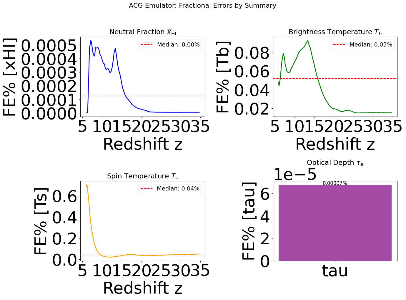
Visualizing Error Statistics

Let’s plot the fractional error as a function of redshift for 1D summaries:

fig, axes = plt.subplots(2, 2, figsize=(14, 10))
rcParams.update({"font.size": 14})

# xHI error vs redshift
axes[0, 0].plot(zs, output_errors.xHI_err.value, "b-", lw=2)
axes[0, 0].set_xlabel("Redshift z")
axes[0, 0].set_ylabel("FE% [xHI]")
axes[0, 0].set_title(r"Neutral Fraction $\overline{x}_{\rm HI}$")
axes[0, 0].axhline(
    np.median(output_errors.xHI_err.value),
    color="r",
    ls="--",
    label=f"Median: {np.median(output_errors.xHI_err.value):.2f}%",
)
axes[0, 0].legend()

# Tb error vs redshift
axes[0, 1].plot(zs, output_errors.Tb_err.value, "g-", lw=2)
axes[0, 1].set_xlabel("Redshift z")
axes[0, 1].set_ylabel("FE% [Tb]")
axes[0, 1].set_title(r"Brightness Temperature $\overline{T}_b$")
axes[0, 1].axhline(
    np.median(output_errors.Tb_err.value),
    color="r",
    ls="--",
    label=f"Median: {np.median(output_errors.Tb_err.value):.2f}%",
)
axes[0, 1].legend()

# Ts error vs redshift
axes[1, 0].plot(zs, output_errors.Ts_err.value, "orange", lw=2)
axes[1, 0].set_xlabel("Redshift z")
axes[1, 0].set_ylabel("FE% [Ts]")
axes[1, 0].set_title(r"Spin Temperature $T_s$")
axes[1, 0].axhline(
    np.median(output_errors.Ts_err.value),
    color="r",
    ls="--",
    label=f"Median: {np.median(output_errors.Ts_err.value):.2f}%",
)
axes[1, 0].legend()

# tau error (scalar)
axes[1, 1].bar(["tau"], [output_errors.tau_err.value], color="purple", alpha=0.7)
axes[1, 1].set_ylabel("FE% [tau]")
axes[1, 1].set_title(r"Optical Depth $\tau_e$")
axes[1, 1].text(
    0,
    output_errors.tau_err.value,
    f"{output_errors.tau_err.value:.5f}%",
    ha="center",
    fontsize=12,
)

plt.suptitle("ACG Emulator: Fractional Errors by Summary", fontsize=16, y=1.02)
plt.tight_layout()
plt.show()

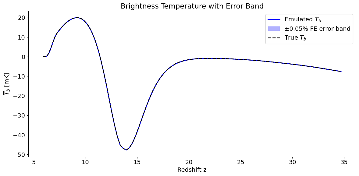
Computing Absolute Errors

The ACG emulator stores fractional errors (FE%). To get absolute errors in physical units, multiply by the output value:

# Convert FE% to absolute errors for plotting with error bands
abs_Tb_err = output_errors.Tb_err.value / 100 * np.abs(Tb_emu)  # Now in mK
abs_xHI_err = output_errors.xHI_err.value / 100 * np.abs(xHI_emu)

# Example plot with error bands
fig, ax = plt.subplots(figsize=(12, 6))

# Plot one sample with error band
sample_idx = 5
ax.plot(zs, Tb_emu[sample_idx], "b-", lw=2, label="Emulated $T_b$")
ax.fill_between(
    zs,
    Tb_emu[sample_idx] - abs_Tb_err[sample_idx],
    Tb_emu[sample_idx] + abs_Tb_err[sample_idx],
    alpha=0.3,
    color="blue",
    label="±0.05% FE error band",
)
ax.plot(zs, Tb_true[sample_idx], "k--", lw=2, label="True $T_b$")

ax.set_xlabel("Redshift z")
ax.set_ylabel(r"$\overline{T}_b$ [mK]")
ax.legend()
ax.set_title("Brightness Temperature with Error Band")
plt.tight_layout()
plt.show()